Distribution transformers worldwide lose an estimated 500 TWh of energy every year. That figure rivals the total electricity consumption of many mid-sized nations. These losses translate directly into higher electricity bills, increased carbon emissions, and wasted fuel at power stations. For these reasons, transformer efficiency has become a central topic in power system engineering, energy regulation, and utility procurement.
Modern power transformers perform remarkably well. Large power transformers rated above 100 MVA routinely achieve efficiencies between 99.5% and 99.7%, while distribution transformers in the 10 kVA to 2500 kVA range operate between 97% and 99%. These numbers make transformers some of the most efficient electrical machines in existence.
In this technical guide, we will discuss how transformer efficiency is defined, what causes losses, how to find the loading point where efficiency is maximum, and how to evaluate a transformer’s performance over a full 24-hour operating cycle.
1. Definition and Mathematical Foundation
Transformer efficiency is the ratio of useful output power to the total input power fed to the device. It tells us how effectively a transformer converts electrical energy from one voltage level to another.
The basic efficiency formula is:
\(\eta=\frac{P_{out}}{P_{in}}\times 100\%\)
where \(\eta\) represents efficiency as a percentage, \(P_{out}\) denotes output power in watts, and \(P_{in}\) is input power in watts.
No transformer is an ideal device. Some energy is always lost during the conversion process, mostly as heat produced by various loss mechanisms. A more practical version of the formula accounts for these losses directly:
\(\eta=\frac{P_{out}}{P_{out}+P_{losses}}\times 100\%\)
This form is especially useful when iron losses and copper losses have been measured separately. The input power is simply the sum of the output power and the total losses.
For a transformer operating at a fractional load \(x\) (where \(x\) is the fraction of full load, ranging from 0 to 1), the efficiency can be written as:
\(\eta_x=\frac{x.S.cos\phi}{x.S.cos\phi\,+\,P_i\,+\,x^2P_c}\times 100\%\)
where \(S\) is the transformer’s rated apparent power in kVA, \(cos\phi\) is the load power factor, \(P_i\) is the iron loss (constant, independent of load), and \(P_c\) is the full-load copper loss.
2. Why do Transformers can Achieve High Efficiency?
Transformers consistently achieve efficiency levels above 95%, with the largest units exceeding 99.5%. Several fundamental characteristics make this possible.
2.1 No Moving Parts
Unlike motors and generators, transformers are static devices. There are no rotating shafts, bearings, or fans required for the core energy conversion process. This eliminates mechanical losses such as friction and windage entirely.
2.2 Efficient Energy Transfer
When alternating current flows through the primary winding, it creates a time-varying magnetic flux in the core. This flux induces a voltage in the secondary winding through mutual inductance. The magnetic coupling between windings avoids any direct electrical connection between circuits and minimises resistive losses that would occur in direct conversion methods.
2.3 Advanced Core Materials
Modern core materials, particularly Cold Rolled Grain Oriented (CRGO) silicon steel, are engineered to minimize magnetic losses. The grain-oriented structure aligns magnetic domains along the preferred flux direction. This alignment reduces hysteresis losses from repeated magnetisation cycles and lowers eddy current losses through high electrical resistivity. The best CRGO grades today achieve core losses as low as 0.9 W/kg at 1.7 Tesla and 50 Hz.
2.4 Low Resistance Windings
Careful winding design using high-conductivity copper conductors with large cross-sectional areas keeps resistive losses small. The copper loss relationship \(P_{cu}=I^2R\) shows that using low-resistance conductors reduces energy waste even when the windings carry large currents.
2.5 Laminated Core Construction
The core is built from thin steel sheets (laminations) rather than a solid block. Each lamination is coated with a thin layer of insulation. This construction breaks up the paths that eddy currents would otherwise follow, suppressing these circulating currents and the heat they generate.
3. Types of Losses in Transformers
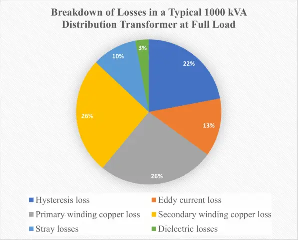
3.1 Iron Losses (Core Losses)
Iron losses, also called core losses or no-load losses occur in the magnetic core and remain constant regardless of load current. These losses are present whenever the transformer is energised, even with no load connected to the secondary winding. They represent a continuous energy drain throughout the transformer’s service life. Iron losses have two distinct components: hysteresis loss and eddy current loss.
3.1.1 Hysteresis Loss
Hysteresis Loss results from the energy needed to repeatedly magnetize and demagnetize the core material as the alternating current reverses direction every cycle. The magnetic domains within the steel must continuously realign with the changing magnetic field. This internal molecular friction releases energy as heat. The Steinmetz equation quantifies hysteresis loss:
\(P_h=K_h f B^n V\)
where, \(P_h\) is hysteresis loss in watts, \(K_h\) is a constant that depends on the core material, \(f\) is frequency in hertz, \(B\) is the maximum flux density in tesla, \(n\) is the Steinmetz exponent (a value between 1.6 and 2.0, commonly around 1.6 for silicon steel), and \(V\) is the core volume.
3.1.2 Eddy Current Loss
Eddy Current Loss arises from circulating currents induced within the conductive core material by the time-varying magnetic flux. According to Faraday’s law, the changing flux induces voltages inside the core itself. These voltages drive closed-loop currents called eddy currents through the steel. The currents flow in paths perpendicular to the flux direction and dissipate energy as \(I^2R\)
The eddy current loss formula is:
\(P_e=K_e t^2 f^2 B^2 V\)
where \(P_e\) is eddy current loss in watts, \(K_e\) is a constant that depends on core material resistivity, \(t\) is lamination thickness in meters.
Notice that eddy current loss depends on the square of frequency, whereas hysteresis loss depends on frequency linearly. This is because the induced voltage (and therefore the circulating current) in each lamination is proportional to the rate of change of flux, which itself increases with frequency. Since the power dissipated by these currents follows the \(I^2R\) relationship, the loss scales with \(f^2\).
For a 50 kVA distribution transformer, iron losses might range from 200 to 300 watts. These losses remain the same whether the transformer runs at no-load or at full-load.
3.2 Copper Losses (Winding Losses)
Copper losses also called winding losses or \(I^2R\) losses result from the electrical resistance of the primary and secondary windings when current flows through them. Unlike iron losses, copper losses vary with the square of the load current. They are load-dependent or variable losses. At no-load, copper loss is zero. At full-load, copper loss reaches its maximum value.
The fundamental relationship governing copper loss is Joule’s law of heating:
\(P_{cu}=I_1^2R_1+I_2^2R_2\)
where\(P_{cu}\) is total copper loss, \(I_1\) and \(I_2\) are primary and secondary currents respectively, and \(R_1\) and \(R_2\) are the resistances of primary and secondary windings. Because of the squared relationship with current, doubling the load current increases copper losses by a factor of four.
When the transformer operates at \(x\) times its rated load (where \(x\) is a fraction between 0 and 1), the copper loss becomes:
\(P_{cu,x}=x^2 P_{cu,FL}\)
where \(P_{cu,FL}\) is the full-load copper loss.
Example: If a transformer has a full-load copper loss of 4 kW, then at half load \((x=0.5)\), the copper loss is \((0.5)^2\times 4=1 \,kW\), only one quarter of the full-load value.
3.3 Stray Losses and Dielectric Losses
Beyond iron and copper losses, transformers experience additional minor losses. Stray losses result from leakage flux that escapes the main magnetic circuit and interacts with structural components such as the tank walls, mounting hardware, and metallic supports. This stray flux induces eddy currents in these conducting structures, which dissipate energy as heat.
Dielectric losses occur in the insulating materials between conductors and between windings. These losses arise from electrical stress on insulation when it is subjected to alternating electric fields. The molecular friction and polarisation effects within the dielectric material produce a small amount of heat. While dielectric losses are small often 1% to 2% of total losses they can increase if insulation quality degrades over time.
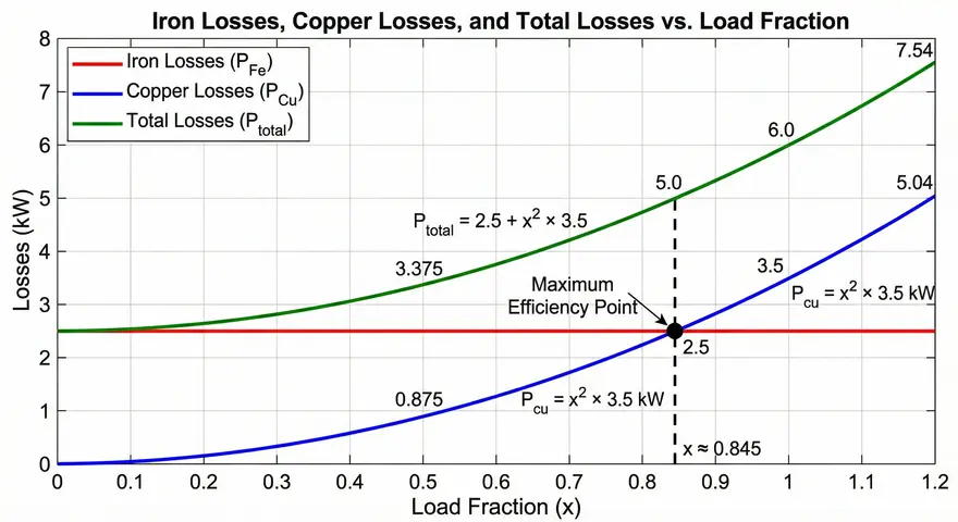
4. Condition for Maximum Efficiency
A transformer reaches its highest efficiency when its constant losses (iron losses) equal its variable losses (copper losses at that loading point). This condition can be derived mathematically.
Starting with the efficiency expression for fractional load \(x\):
\(\eta=\frac{x.S.cos\phi}{x.S.cos\phi\,+\,P_i\,+\,x^2 P_c}\)
To find the maximum, we can rewrite efficiency as:
\(\eta=\frac{1}{1+\dfrac{P_i + x^2 P_c}{x.S.cos\phi}}\)
Efficiency is maximised when the fraction \(\frac{P_i + x^2 P_c}{x.S.cos\phi}\) is minimized. Since \(S.cos\phi\) is a constant for a given load power factor, we need to minimize:
\(L(x)=\frac{P-i}{x}+x.P_c\)
Taking the derivative with respect to \(x\) and setting it to zero:
\(\frac{dL}{dx}=-\frac{P_i}{x^2}+P_c=0\)
Solving,
\(P_c=\frac{P_i}{x^2}\)
\(x^2P_c=P_i\)
Therefore, maximum efficiency occurs when:
\(x=\sqrt{\frac{P_i}{P_c}}\)
The load fraction for maximum efficiency equals the square root of the ratio of iron losses to full-load copper losses.
Example: If a transformer has iron losses of 1.5 kW and full-load copper losses of 6 kW, maximum efficiency occurs at:
\(x=\sqrt{\frac{1.5}{6}}=\sqrt{0.25}=0.5\)
This means the transformer operates most efficiently at 50% of its rated load not at full load. This result has practical consequences for transformer selection. If a load is expected to average around 200 kVA, choosing a 400 kVA transformer (so it runs near 50% loading) may yield better long-term efficiency than a 250 kVA unit running near 80%.
5. All-Day Efficiency of a Transformer
Standard efficiency calculated at a single loading point does not tell the full story for distribution transformers. These transformers remain connected to the grid 24 hours a day but experience widely varying loads with heavy loading during daytime peak hours and light loading at night. Iron losses accumulate for every hour the transformer is energised, regardless of load. A transformer that looks efficient at full load may waste energy over a full day if it spends most hours lightly loaded.
All-day efficiency (also called energy efficiency) is the ratio of total energy output to total energy input over a complete 24-hour period:
\(\eta_{all-day}=\frac{\text{Energy output (kWh) in 24 hours}}{\text{Energy input (kWh) in 24 hours}} \times 100\%\)
This can be expanded to show the individual loss contributions:
\(\eta_{all-day}=\frac{\sum (kW_{out} \times hours)}{\sum(kW_{out} \times hours)\,+\,(P_i \times 24)+\sum(P_{cu}\times hours)}\times 100\%\)
where \(P_i\) is the constant iron loss present for all 24 hours, and \(\sum(P_{cu}\times hours)\) is the accumulated copper loss energy, which varies with the load pattern.
5.1 Calculation Example of All Day Efficiency of a Transformer
To illustrate all-day efficiency calculation, consider a 400 kVA distribution transformer with the following characteristics:
- Full-load iron losses = 2.5 kW
- Full-load copper losses = 3.5 kW
The transformer follows this 24-hour load cycle:
| Period | Duration | Load (kW) | Power Factor |
|---|---|---|---|
| 1 | 6 hours | 300 | 0.8 |
| 2 | 10 hours | 200 | 0.7 |
| 3 | 4 hours | 100 | 0.9 |
| 4 | 4 hours | 50 | 0.95 |
Period 1 (6 hours, 300 kW at 0.8 pf):
- \(kVA = \frac{300}{0.8} = 375 kVA\)
- Load fraction \(x_1=\frac{375}{400}=0.9375\)
- Copper loss = \((0.9375)^2\times 3.5=3.08 kW\)
- Energy output =\(300\times 6=1800 kWh\)
- Copper loss energy =\(3.08\times 6=18.48kWh\)
Period 2 (10 hours, 200 kW at 0.7 pf):
- kVA = \(\frac{200}{0.7} = 285.7 kVA\)
- Load fraction\(x_2=\frac{285.7}{400}=0.714\)
- Copper loss =\((0.714)^2\times 3.5=1.78 kW\)
- Energy output = \(200\times 10=2000 kWh\)
- Copper loss energy =\(1.78\times 10=17.8 kWh\)
Period 3 (4 hours, 100 kW at 0.9 pf):
- kVA = \(\frac{100}{0.9} = 111.1 kVA\)
- Load fraction \(x_3=\frac{111.1}{400}=0.278\)
- Copper loss = \((0.278)^2\times 3.5=0.27 kW\)
- Energy output = \(100\times 4=400 kWh\)
- Copper loss energy = \(0.27\times 4=1.08 kWh\)
Period 4 (4 hours, 50 kW at 0.95 pf):
- kVA = \(\frac{50}{0.95} = 52.6 kVA\)
- Load fraction \(x_4=\frac{52.6}{400}=0.132\)
- Copper loss = \((0.132)^2\times 3.5=0.06 kW\)
- Energy output = \(50\times 4 =200 kWh\)
- Copper loss energy = \(0.06\times 4= 0.24 kWh\)
Total energy calculations:
- Total energy output \(= 1800 + 2000 + 400 + 200 = 4400 kWh\)
- Total iron loss energy \(= 2.5 \times 24 = 60\, kWh\) (constant for entire 24 hours)
- Total copper loss energy \(= 18.48 + 17.8 + 1.08 + 0.24 = 37.6 kWh\)
- Total loss energy \(= 60 + 37.6 = 97.6 kWh\)
All-day efficiency:
\(\eta_{all-day}=\frac{4400}{4400+97.6}\times 100=\frac{4400}{4497.6}\times 100 = 97.83\%\)
Now let us compare this with the full-load efficiency at unity power factor:
\(\eta_{FL}=\frac{400}{400+2.5+3.5}\times 100=\frac{400}{406}\times 100 = 98.52\%\)
The all-day efficiency of 97.83% is lower than the full-load efficiency of 98.52%. This gap exists because iron losses run for all 24 hours while the transformer operates at partial load for most of the day. The iron losses have a disproportionate effect on energy efficiency when the average load is well below rated capacity.
This is exactly why utilities and regulators pay special attention to no-load losses when selecting distribution transformers. Reducing iron losses even by a small amount saves energy every hour of every day for the 25–30 year service life of the transformer.
6. Factors Affecting Transformer Efficiency
6.1 Load Conditions
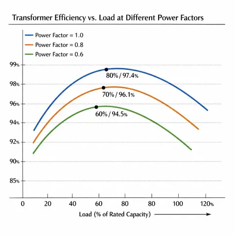
The load magnitude has a strong influence on transformer efficiency. The efficiency curve has a characteristic shape — it starts low at light loads, rises to a peak at the optimal loading point, and then gradually declines at heavier loads.
At very light loads (10–30% of rated capacity), efficiency is low because the constant iron losses dominate while useful output power is small. As loading increases toward the optimal point — where copper losses equal iron losses — efficiency rises because output power grows faster than the variable copper losses. For distribution transformers, this optimal point is often in the 50–70% loading range. For power transformers, it falls closer to 70–90%.
Beyond the peak, efficiency drops gradually because copper losses grow with the square of the current while output power increases only linearly. At overload conditions (above 100% rated capacity), the drop becomes more pronounced as excessive copper losses and effects like increased core saturation add further losses.
6.2 Power Factor
Power factor also affects efficiency at a given kVA loading. Consider a transformer delivering 80 kW. At unity power factor, this requires 80 kVA and a certain current level. At 0.8 power factor, delivering the same 80 kW requires 100 kVA and 25% more current. The higher current produces higher copper losses. So for constant real power output, efficiency falls as power factor decreases.
For any given loading level, the highest efficiency occurs at unity power factor. Efficiency drops progressively as power factor decreases. This is one reason why power factor correction is so important in industrial plants where motors and other inductive loads naturally produce lagging power factors.
6.3 Operating Temperature
Temperature affects transformer efficiency through its influence on winding resistance. Copper’s resistance increases by approximately 0.393% per degree Celsius. As a transformer heats up during operation, this resistance increase raises copper losses directly.
Example: A transformer operating at 105°C (75°C above a 30°C ambient) has a winding resistance about 33% higher than at the 20°C reference temperature:
\(R_{105}=R_{20}\times [1+0.00393\times (105−20)] = R_{20}×1.334\)
This 33% increase in resistance translates directly to 33% higher copper losses at the same current. Effective cooling system design through natural oil circulation, forced oil pumps, or external fans helps keep temperatures lower and preserves efficiency.
6.4 Core Material Selection
The choice of core material is one of the most impactful design decisions for transformer efficiency because it directly controls iron losses. These losses run continuously for the entire service life of the transformer.
CRGO Silicon Steel is the industry standard for power and distribution transformers. The grain-oriented structure aligns magnetic domains along the rolling direction, which corresponds to the flux path in the finished core. This alignment reduces hysteresis losses by lowering the energy needed to reorient domains during each magnetisation cycle. The addition of 2–4% silicon raises electrical resistivity, which suppresses eddy currents. Modern CRGO grades achieve specific core losses of 0.9–1.1 W/kg at 1.7 Tesla and 50 Hz. Older non-oriented steels had losses of 2–4 W/kg under the same conditions — a dramatic difference.
6.5 Design and Construction Quality
Many detailed design and manufacturing decisions affect the final efficiency of a transformer.
6.5.1 Winding Conductor Selection
Winding conductor selection involves choosing between copper and aluminium. Copper has about 61% higher electrical conductivity than aluminium. To carry the same rated current, aluminium windings need roughly 60% more cross-sectional area, resulting in larger and heavier coils despite aluminium’s lower density. Copper windings produce lower losses for a given physical size, but their higher cost leads some manufacturers to use aluminium in cost-sensitive applications.
6.5.2 Core Construction Quality
Core construction quality matters because gaps and imperfections in the magnetic circuit cause localised flux concentrations and increased losses. Precise cutting and stacking of laminations reduces these effects. Lamination thickness directly impacts eddy current losses. Thinner laminations reduce eddy currents but require more careful handling during assembly.
6.5.3 Core Joint Design
Core joint design influences both losses and magnetising current. Step-lap joints, where successive laminations overlap in staggered patterns, provide better magnetic continuity than simple butt joints. This reduces localised flux concentrations at the joints. Premium transformers use carefully engineered step-lap patterns, while economy designs may use simpler butt joints.
6.5.4 Cooling System Design
Cooling system design affects efficiency indirectly by managing operating temperature. Oil-immersed transformers rely on circulating oil and external radiators to remove heat. The design of radiators, oil flow paths, and oil quality all affect heat removal. Large power transformers often use forced oil and forced air cooling (OFAF) to maintain lower winding temperatures and preserve efficiency under heavy loading.
6.5.5 Insulation System Quality
Insulation system quality affects dielectric losses and long-term reliability. While dielectric losses are small (1–2% of total losses in a healthy transformer), degraded insulation can increase these losses and eventually lead to failure. High-quality insulating materials with low dissipation factors keep dielectric losses to a minimum.
7. Efficiency Testing
The iron losses and copper losses used in efficiency calculations are not measured by loading the transformer to full power and measuring input and output directly. For large transformers, this would require enormous amounts of power and load equipment. Instead, two simple tests provide all the data needed.
The open-circuit (no-load) test measures iron losses. The secondary winding is left open (no load connected), and rated voltage is applied to the primary winding. The small current that flows called the no-load current supplies only the iron losses and the magnetising current. A wattmeter on the primary side reads the iron loss directly, since copper losses are negligible at this small current.
The short-circuit test measures copper losses. The secondary winding is short-circuited through an ammeter, and a reduced voltage is applied to the primary — just enough to circulate full-load current through the windings. At this reduced voltage (usually 5–10% of rated voltage), the core flux is very low and iron losses are negligible. The wattmeter reading gives the full-load copper loss directly.
These two tests, combined with the efficiency formulas presented earlier, allow engineers to calculate efficiency at any load and power factor without ever needing to supply or absorb the full rated power of the transformer.
8. Efficiency Standards and Regulations
Governments and international bodies have established minimum efficiency standards for transformers, recognizing the enormous energy savings possible across millions of installed units.
- IEC 60076-20 specifies methods for measuring and declaring energy performance of power transformers. It defines efficiency tiers and provides a common framework for comparing transformers from different manufacturers.
- The EU Ecodesign Directive introduced mandatory minimum efficiency requirements for power transformers in two tiers. Tier 1 took effect in 2015 and Tier 2 in 2021, each setting progressively tighter limits on no-load and load losses.
- The US Department of Energy (DOE) has set minimum efficiency standards for liquid-immersed and dry-type distribution transformers, updated periodically to reflect improvements in available technology.
- IEEE C57.12.00 and related standards in the United States define testing procedures, tolerance limits, and performance specifications for power and distribution transformers.
- India’s IS 1180 governs distribution transformer specifications, and the Bureau of Energy Efficiency (BEE) operates a star rating programme that labels transformers from 1 to 5 stars based on their loss performance.
9. Conclusion
Transformer efficiency is governed by two main loss categories: iron losses that run constantly and copper losses that vary with the square of the load current. Maximum efficiency occurs at the specific loading point where these two loss categories are equal. A point that can be calculated using \(x=\sqrt{\frac{P_i}{P_c}}\) and used to guide transformer selection for a given application.
For distribution transformers that operate around the clock at varying loads, all-day efficiency provides a more honest measure of performance than a single full-load efficiency number. As the calculation example in this article shows, iron losses accumulate relentlessly and can dominate total energy losses over a 24-hour cycle.
10. Frequently Asked Questions (FAQs)
Transformer efficiency is the percentage of input power that reaches the load as useful output power. The remaining power is lost as heat through core losses and winding losses inside the transformer.
The basic formula is η = (Output Power / Input Power) × 100%. A more practical version is η = Output Power / (Output Power + Total Losses) × 100%, which separates iron and copper losses.
Every transformer has unavoidable losses including hysteresis and eddy currents in the core, resistive heating in the windings, stray flux losses, and dielectric losses in insulation. These losses always consume some input energy.
Iron losses occur in the magnetic core due to hysteresis and eddy currents. They remain constant at all load levels and are present whenever the transformer is energised, even at no load.
Copper losses are heating losses in the primary and secondary windings. They vary with the square of the load current, zero at no load and maximum at full load.
Hysteresis loss is the energy spent reversing magnetic domains in the core material during each AC cycle. It depends on the core material, flux density, and supply frequency.
Eddy current loss comes from small circulating currents induced inside the core by the changing magnetic flux. Laminating the core into thin insulated sheets reduces these currents.
Lamination breaks the core into thin insulated sheets, which interrupts eddy current paths. Thinner laminations force eddy currents into smaller loops, reducing their magnitude and the associated heat loss.
A transformer reaches maximum efficiency when its iron losses equal its copper losses.
Not always. Most distribution transformers reach peak efficiency between 50% and 70% of rated load. The exact point depends on the ratio of iron losses to copper losses for that specific design.
All-day efficiency is the ratio of total energy output to total energy input over a full 24-hour period. It accounts for varying loads throughout the day and gives a more realistic performance measure.
Iron losses accumulate for all 24 hours regardless of load. During light-load hours, these constant losses form a large fraction of the total input energy, pulling the overall energy efficiency down.