Distance protection is one of the most widely used and reliable methods for protecting transmission lines in modern power systems. Unlike overcurrent relays that operate based solely on current magnitude, distance relays measure the impedance between the relay location and the fault point on the transmission line. This enables fast, selective, and coordinated protection across the entire power network.
The principle is based on Ohm’s law: by measuring the voltage and current at the relay location, we can calculate the impedance to the fault point, fault distance and determine whether the fault lies within a predetermined protection zone.
Why Do We Need Distance Protection?
Transmission lines are the backbone of electrical power systems, carrying electricity over long distances from generation stations to distribution centers. These lines are constantly exposed to various faults such as short circuits between phases (phase-to-phase faults), ground faults (phase-to-ground faults), double line-to-ground faults, and three-phase faults.
When a fault occurs, extremely high currents flow through the system, which can cause permanent damage to equipment, cascading failures across the network, power blackouts affecting millions of consumers, and fire hazards.
Therefore, we need a fast, accurate, and selective protection scheme that can detect the fault immediately, isolate only the faulty section, determines the distance of fault location, keep the rest of the system operational, and minimize damage and service interruption.
Limitations of Other Protection Methods
Before understanding why distance protection is superior for Transmission Lines, it’s important to examine other traditional methods and its limitations.
Overcurrent protection operates solely on the magnitude of current flowing through the relay. However, fault current depends on several factors, including source impedance, network configuration, and the exact fault location. Because of this, it is difficult to achieve both fast and selective protection on long transmission lines using overcurrent relays alone. Current magnitude by itself cannot reliably indicate where along the line the fault has occurred.
Differential protection offers highly sensitive and selective protection by comparing currents at both ends of the Transmission Line. While very effective, it requires reliable communication channels between line ends and is therefore more complex and expensive to apply on every transmission line, especially over long distances or in wide-area networks.
Distance protection overcomes these drawbacks and adds a major practical advantage. It not only detects and clears faults quickly, but also estimates the distance to the fault using measured impedance. This distance-to-fault information is displayed on the relay HMI or sent to the SCADA system, allowing operators and maintenance teams to know exactly which line section or tower span to inspect.
In contrast, overcurrent and differential relays simply indicate that a fault has occurred and tripped the line, without providing any direct indication of fault location or where to begin patrolling, making post-fault field work slower and less efficient.
Fundamental Principle of Distance Protection
The distance relay measures the apparent impedance (Z) seen from the relay terminal toward the fault point. Using the fundamental electrical relationship:
\(Z = \frac{V}{I}\)
Where:
- \(Z\) = Apparent impedance to the fault point
- \(V\) = Voltage measured at the relay location
- \(I\) = Current flowing through the relay
How Distance Protection Works
Consider a simple transmission line with a relay at the sending end. When a fault occurs at distance ‘d’ from the relay, the relay measures voltage (V) and current (I) at its location, calculates impedance using Z = V/I, and since the line impedance is known (R + jX per unit length), the distance can be calculated as:
\(\text{Distance to fault (d)} = \frac{Z_{measured}}{Z_{\text{per unit length}}}\)
For example, if the line impedance is 0.4 Ω/km and the measured impedance is 40 Ω, then the distance would be
\(\text{Distance to fault (d)} = \frac{Z_{measured}}{Z_{\text{per unit length}}}=\frac{40}{0.4} = 100 \text{km}\)
This simple yet elegant principle forms the basis of all distance protection schemes used worldwide in transmission systems.
Three Zones of Distance Protection
The most important feature of distance protection is the three-zone concept, which provides both primary and backup protection with definite time delays. Each zone serves a specific purpose in the overall protection strategy.
Zone 1 (Instantaneous Protection)
| Parameter | Value |
|---|---|
| Coverage | 80-85% of protected line length |
| Reach Setting (Z₁) | 0.8 × Z_line |
| Time Delay | 0 ms (Instantaneous) |
| Purpose | Primary protection for most of the line |
| Advantage | Fast clearing reduces system stress |
Zone 1 covers approximately 80% of the transmission line and reaches 80% because we need a safety margin to avoid maloperation beyond the protected line. This zone operates instantaneously with zero millisecond delay, protecting the line from the sending end up to 80% of its length.
The 80% reach is not arbitrary, it is carefully chosen to protect the vast majority of the line while maintaining a safety margin to prevent false trips for external faults that might occur slightly beyond the line end.
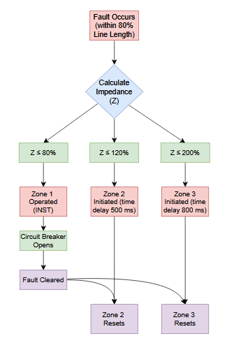
For example, for a 200 km line, Zone 1 reaches 0.8 × 200 = 160 km. If any fault occurs within the 160 km range, the Zone 1 element of the Distance Relay picks up and it sends trip signal to the Circuit Breaker associated with the line instantaneously in approximately 20-50 milliseconds, which is fast enough to prevent damage to equipment and preserve system stability.
Zone 2 (Primary Backup)
| Parameter | Value |
|---|---|
| Coverage | 100% of protected line + 20% of adjacent line |
| Reach Setting (Z₂) | 1.2 × Z_line |
| Time Delay | 0.3 – 0.5 seconds |
| Purpose | Backup for near-end faults + primary for adjacent line faults |
| Advantage | Protects against Zone 1 failure |
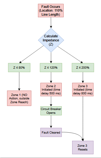
Zone 2 extends to 100% of the protected line and 20% into the next line, providing total 120% coverage with a time delay of 0.3-0.5 seconds.
The reason for including 20% of the adjacent line in the reach is to coordinate with the Zone 1 of the adjacent relay. If a fault occurs on the next line, the adjacent line’s relay Zone 1 should clear it first. If the adjacent relay fails, this relay’s Zone 2 provides backup protection with a slight time delay to allow the primary relay time to operate.
This zone acts as a backup if Zone 1 fails to clear a fault so that no fault near the end of the protected line goes uncleared. Additionally, Zone 2 provides primary protection for the adjacent transmission line, working in coordination with its own distance relay.
For example, for a 200 km line, Zone 2 reaches 1.2 × 200 = 240 km with a trip time of 0.3-0.5 seconds. This time delay is critical for coordination; it ensures that if Zone 1 of the same relay operates for some reason during a fault on the adjacent line, that Zone 1 will clear the fault before Zone 2 has a chance to operate.
Zone 3 (Remote Backup)
| Parameter | Value |
|---|---|
| Coverage | 100% of protected line + 100% of one or more adjacent lines |
| Reach Setting (Z₃) | 2 × Z_line or beyond |
| Time Delay | 0.8 – 1.0 seconds or more |
| Purpose | Backup for upstream or remote faults |
| Advantage | Ultimate backup protection |
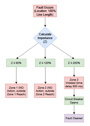
Zone 3 extends beyond Zone 2 to remote sections of the network, providing the ultimate backup protection with the longest time delay of 0.8-1.0 seconds or more. This zone provides coordinated backup for remote faults that might occur far in the network. The extended reach of Zone 3 ensures that even if multiple relays in the network fails, this relay will eventually clear the fault and prevent cascading failures that could spread throughout the network.
For example, for a 200 km line, Zone 3 reaches 2 × 200 = 400 km or beyond with a trip time of 0.8-1.0 seconds.
Zone 3 must be carefully set to avoid false trips that could inadvertently disconnect healthy portions of the network. The long time delay of Zone 3 ensures that many relays in the network have the opportunity to clear the fault before this relay operates.
If a fault occurs on the second line downstream, the first downstream relay’s Zone 1 should clear it immediately, the second downstream relay’s Zone 2 should clear it next, and this relay’s Zone 3 provides final backup.
Relay Characteristics: R-X Impedance Diagram
Distance relays don’t operate on a simple circular boundary. Instead, they use different geometric shapes on the R-X plane (complex impedance diagram) to define protection zones.
The R-X Impedance Plane
The R-X diagram is a 2D representation where the vertical axis (X) represents reactance (Ω) which is the imaginary part of impedance, the horizontal axis (R) represents resistance (Ω) which is the real part of impedance, and each point on the plane represents an impedance value.
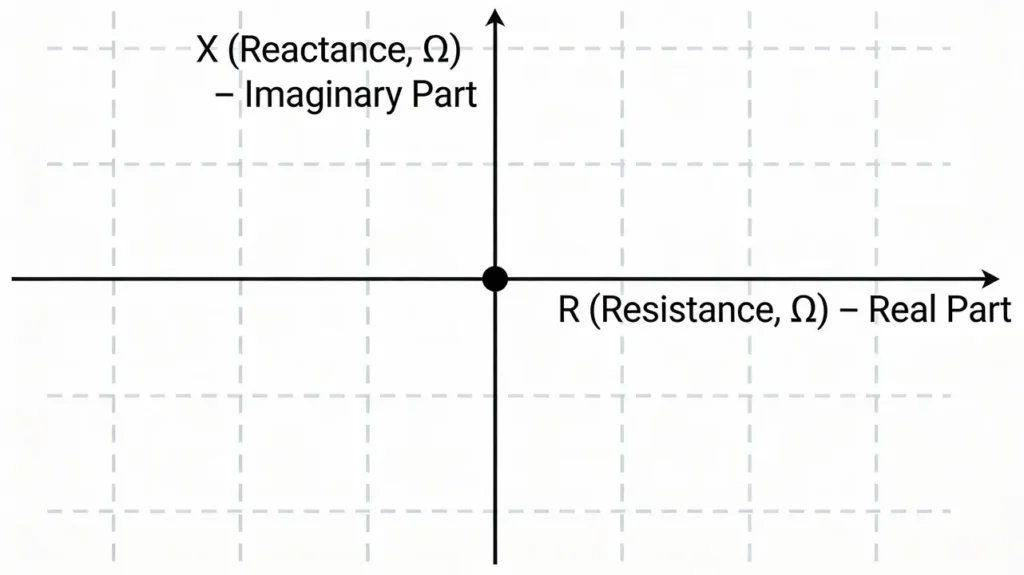
Every impedance, whether from normal load flow or a fault condition, can be plotted as a single point on this two-dimensional plane. Transmission line impedances are plotted as points on this plane. When a fault occurs, the measured impedance point will move on this diagram, and the relay checks whether this point falls within its trip boundary.
The R-X plane is useful for understanding relay operation. When a fault occurs near the relay, the impedance point plots close to the origin. As the fault location moves farther away, the impedance point moves outward from the origin. The relay trip boundary is drawn on this plane as a closed curve, circle, or polygon, and any impedance point inside this boundary causes a trip. This visual representation makes it easy to understand why certain conditions cause trips and others don’t.
Types of Relay Characteristics
1. Circular (Mho) Characteristic
The Mho characteristic appears as a circle on the R-X diagram, which has several distinct advantages.
The Mho characteristics provides good directional discrimination, allowing the relay to distinguish between faults in different directions.
It also has natural immunity to power swings that occur during large system disturbances. During a power swing, the impedance oscillates back and forth on the R-X plane. The Mho characteristic’s circular shape allows it to naturally “miss” these oscillating impedance points while catching steady-state fault impedances.
The Mho characteristic has a simple and reliable design that has been proven effective for decades in protection schemes. The mathematics behind the Mho circle is straightforward, and the implementation is straightforward enough that electromagnetic relays could achieve it with simple mechanical designs.
However, the Mho characteristic does have some limitations. It has limited resistance reach, meaning it may not adequately protect against high impedance faults involving significant arc resistance. Since the circle is centered on the origin, it naturally covers more reactance distance than resistance distance, which is appropriate for typical transmission lines but can miss arcing faults.
It may also have blindness to certain fault types under specific system conditions. For example, the circle’s geometry might not extend far enough in the resistance direction to cover all possible high impedance faults.
Despite these limitations, the Mho characteristic remains the most commonly used for distance protection of high-voltage transmission lines due to its overall reliability and directional properties.
2. Quadrilateral Characteristic
The Quadrilateral characteristic appears as a rectangular shape on the R-X diagram, offering different advantages compared to the Mho shape.
Advantages:
- Better resistance reach
- Can cover high impedance faults
- Flexible shape for specific protection needs
Disadvantages:
- More complex logic
- Sensitive to parameter variations
- Requires careful setting
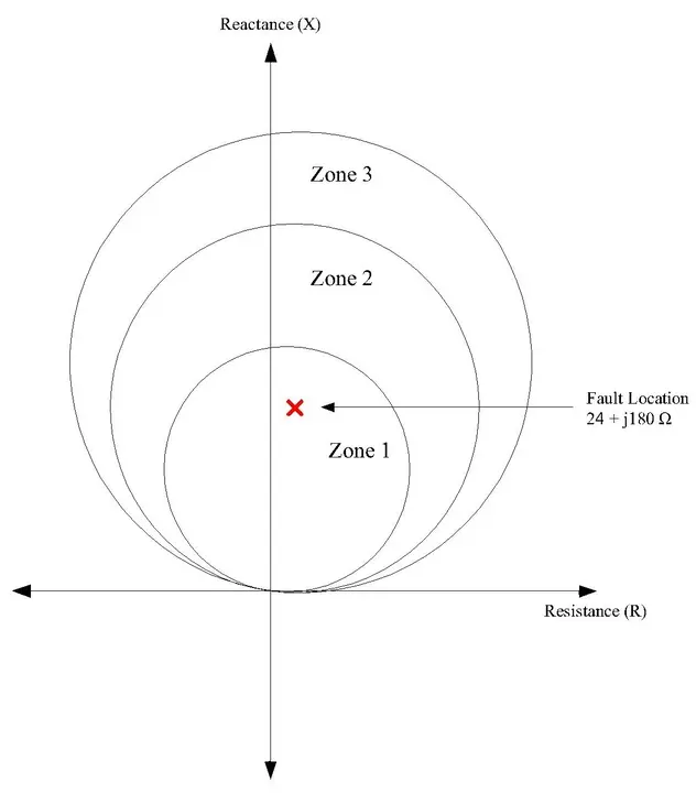
Practical Example: Zone 1 and Zone 2 on R-X Diagram
For a 220 kV transmission line with a total line impedance of 40 + j300 Ω, Zone 1 is set for 80% reach: 0.8 × (40 + j300) = 32 + j240 Ω with a trip time of 0 ms.
This point plots at R = 32, X = 240 on the R-X diagram. The Zone 1 circle is drawn with its boundary passing through this point and extending to cover fault impedances within 80% of the line length.
Zone 2 is set for 120% reach: 1.2 × (40 + j300) = 48 + j360 Ω with a trip time of 0.4 seconds. This point plots at R = 48, X = 360. The Zone 2 circle is larger than the Zone 1 circle, encompassing all of Zone 1 and extending beyond it.
These points plot as circles on the R-X diagram, with the inner circle representing Zone 1’s instantaneous protection and the outer circle representing Zone 2’s time-delayed backup protection.

When a fault occurs on the transmission line, the measured impedance point appears on the R-X diagram. If it falls inside the Zone 1 circle, the relay trips immediately. If it falls between the Zone 1 and Zone 2 circles, the relay waits 0.4 seconds, during which time the measured impedance should remain in that region if it is truly a fault. If it remains in Zone 2 after 0.4 seconds, the relay trips; if the impedance point exits Zone 2 (indicating a power swing), the relay will not trip.
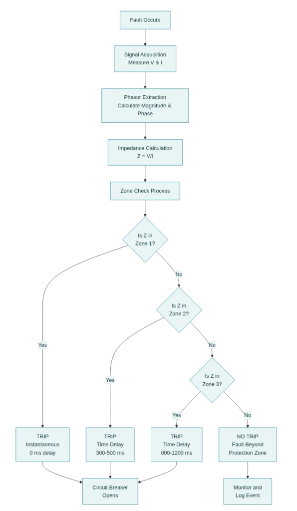
Distance Protection Operating Logic
Step-by-Step Operation
The distance relay operates through a systematic sequence that ensures accurate and timely fault detection and isolation.
Step 1: Signal Acquisition
The first step is Signal Acquisition, where voltage is measured via potential transformers and current is measured via current transformers, then both signals undergo analog-to-digital conversion and signal processing to prepare them for analysis.
The analog signals are sampled at high frequency (typically 1-4 kHz) to capture the waveform details accurately.
Step 2: Phasor Extraction
The second step is Phasor Extraction, where the relay extracts the magnitude and phase angle of voltage and current. The relay uses FFT (Fast Fourier Transform) or Fourier analysis for precise measurements, and separates positive, negative, and zero-sequence components to identify the fault type.
This decomposition is important because different fault types have different patterns of sequence components. A single line-to-ground fault has significant zero-sequence current, while a phase-to-phase fault has no zero-sequence current at all.
Step 3: Impedance Calculation
The third step is Impedance Calculation, where for phase-to-phase faults the relay calculates
\(Z = \frac{V_{phase}}{I_{phase}}\)
For phase-to-ground faults it uses
\(Z = \frac{V_{phase}}{(I_{phase} + k₀I₀)}\)
Where, \(k₀\) is the compensation factor and \(I₀\) is zero-sequence current.
The compensation factor accounts for the different impedance of the zero-sequence path through the ground, which is different from the positive-sequence path through the air. Without proper compensation, the relay would misinterpret ground faults.
Step 4: Fault Detection
The fourth step is Fault Detection, where the relay checks if measured impedance is within Zone 1 boundary and sends an instant trip signal if yes.
If not, it checks Zone 2 and Zone 3 with a time delays.
Step 5: Fault Classification
The fifth step is Fault Classification, where the relay determines the fault type (single line-to-ground, double line-to-ground, phase-to-phase, or three-phase).
Based on the pattern of zero-sequence current, negative-sequence current, and which phases have high current, the relay identifies exactly which phase or phases are faulted.
This allows it to use the appropriate impedance formula and send selective trip to relevant breaker pole(s).
Step 6: Tripping Decision
The sixth step is Tripping Decision, which follows a clear logic.
If impedance is within Zone 1, the relay sends a TRIP command immediately with 0 ms delay. The relay output contact energizes an output relay or programmable logic controller that trips the circuit breaker instantly.
If impedance is within Zone 2, the relay starts a timer for 0.3-0.5 seconds and sends a TRIP command if impedance remains in Zone 2 after the delay. This allows time for upstream relays to clear external faults.
If impedance is within Zone 3, the relay starts a timer for 0.8-1.0 seconds and sends a TRIP command if impedance remains in Zone 3 after the delay. This provides ultimate backup for remote faults.
If impedance is outside all zones, the relay sends NO TRIP signal because the fault is external to the protected line and should be handled by the protection system of that external line.
Advantages of Distance Protection
1. Speed
Zone 1 operates instantaneously with zero millisecond delay, while other zones have definite time delays. This makes distance protection much faster than traditional overcurrent relays, which typically require several cycles to operate.
When a fault occurs, every millisecond matters. The heat generated in a fault is proportional to the square of the current multiplied by the time the current flows. Even a 50 millisecond reduction in fault clearing time can reduce the thermal energy delivered to faulted equipment by 30-50%.
2. Selectivity
Distance protection operates based on distance, not just current magnitude, giving it superior selectivity compared to other protection methods. This distance-based discrimination allows the relay to clearly distinguish between faults on different lines. A fault 100 km away has very different impedance than a fault 1 km away, so the relay can easily tell them apart even if they produce similar currents.
The selectivity enables it to coordinate well with neighboring relays because each relay knows its protected line and the extent of its responsibility.
The selectivity is so effective that it avoids unnecessary tripping of adjacent equipment. When a fault occurs on a given transmission line, only that line is disconnected; all adjacent lines continue operating normally.
3. Reliability
Distance protection works effectively even with varying system conditions and changing network configurations. The protection operates independently and requires only local measurements of voltage and current, eliminating the need for communication with other devices for primary protection.
This independence makes distance protection inherently reliable; it does not depend on external communication channels that might fail or be unavailable.
4. Economy
A single distance protection device provides multiple zones of protection, eliminating the need for separate devices for primary and backup protection. This reduces the need for expensive pilot schemes or communication-based schemes for primary protection, resulting in lower installation and maintenance costs.
5. Flexibility
Distance protection can be adapted for different line configurations, whether radial, looped, or meshed networks. The relay offers multiple characteristic shapes including Mho, Quadrilateral, and other options, allowing engineers to select the best choice for specific applications.
The settings are easy to adjust for system changes such as line upgrades or network reconfigurations. Simply reprogramming a few constants in the relay adapts it to the new system.
The device can be upgraded with modern algorithms to handle emerging challenges such as inverter-based renewable energy or FACTS controllers.
Factors Affecting Distance Protection Measurement
1. Power Swing
Power swing occurs during large disturbances when the system loses synchronism temporarily. During a power swing, the impedance seen by the relay oscillates back and forth rather than reaching a steady state. An oscillating impedance signal can trigger false trips if the relay is not properly protected.
The solution to this problem is the implementation of Power Swing Blocking (PSB) schemes that detect the characteristic oscillating pattern.
The relay blocks distance elements when a power swing is detected and resumes normal operation when the swing dies out and system stability returns.
Power swing detection can work by watching the impedance trajectory. If the impedance point traces a path on the R-X diagram that goes around in circles or spirals, this is definitely a power swing. If it moves rapidly to a fixed point, this indicates a fault.
2. Load Encroachment
Load encroachment occurs when the load impedance approaches or falls within the relay characteristic during heavy load conditions. Since the load impedance point moves within the R-X diagram during normal operation, during extremely heavy loading conditions it can approach the relay’s trip boundary and cause unwanted trips.
The solution involves load encroachment blocking schemes that prevent trips during normal load flow by analyzing the voltage phase angle or monitoring reactive power.
These schemes recognize the characteristics that distinguish load flow from actual faults. During normal load flow, the current lags the voltage by the angle of the load impedance. During a fault, the voltage at the relay location drops while the current increases. These patterns are completely different, allowing the relay to distinguish between them even if the impedance values are similar.
Advanced schemes monitor power flow direction and can tell the difference between power flowing through the line (load condition) and power injected at the fault point (fault condition).
3. Arc Resistance
For example, a fault at 50 km with 50 Ω arc resistance might appear as only 45 km to the relay.
Non-metallic faults such as lines down on trees or insulators with tracking create an arc with significant resistance. This arc resistance increases the measured impedance significantly compared to a pure metallic fault. This can cause the relay to underreach, calculating a shorter distance to the fault than actually exists.
The solution is to increase the resistance reach (R-reach) of the relay characteristic to cover impedances that include arc resistances. Engineers can estimate the maximum arc resistance for the line’s environment and ensure the relay’s R-reach extends at least that far.
4. Mutual Coupling
When two transmission lines share the same tower or run parallel to each other, the magnetic field generated by current in one line couples with the other line through mutual inductance. This mutual coupling affects the impedance measurement made by the distance relay, causing errors in the calculated distance to fault.
The solution is to apply compensation factors to the relay algorithm that account for mutual impedance effects. These factors can be calculated based on the line configuration and incorporated into the distance calculation formula to correct for coupling errors. The relay can use the current from the parallel line (measured at a remote location and communicated to the relay) to correct for mutual coupling.
5. Series Compensating Capacitors
Series capacitors are installed on transmission lines to increase the power transfer capability and improve system stability by reducing the apparent series reactance of the line. However, they introduce complexity in the impedance that the relay sees.
When a capacitor is inserted into the line, it reduces the apparent impedance, causing the relay to measure impedance less than the actual distance to fault. The capacitor inserts negative reactance (capacitive reactance) that partially cancels the positive reactance (inductive reactance) of the line. This causes the relay to underreach and fail to detect faults near the capacitor location.
The solution is to use adaptive algorithms that detect when a capacitor has been inserted and adjust the relay characteristic accordingly. Modern digital relays can detect when a capacitor is in service by analyzing the rate of change of impedance or by receiving control signals from the capacitor control system. Once the relay knows the capacitor is active, it can add back the known capacitor impedance to the measured impedance to calculate the true distance to fault.
Distance Protection Algorithm: Mathematical Foundation
Basic Impedance Calculation
For a phase-to-ground fault, the distance relay calculates impedance using a special formula that accounts for the zero-sequence effects:
\(Z = \frac{V_{phase}}{(I_{phase} + k₀ × I₀)}\)
Where:
- \(V_{phase}\) = Phase voltage phasor
- \(I_{phase}\) = Phase current phasor
- \(I₀\) = Zero-sequence current
- \(k₀\) = Zero-sequence compensation factor = \(\frac{(Z₀ – Z₁)}{Z₁}\)
The zero-sequence impedance (Z₀) is the impedance of the path through the ground return, which is typically much larger than the positive-sequence impedance (Z₁). The compensation factor accounts for this difference.
For a phase-to-phase fault, the calculation is simpler:
\(Z = \frac{ΔV}{ΔI} = \frac{(V_{\text{phase A}} – V_{\text{phase B}})}{(I_{\text{phase A}} – I_{\text{phase B}})}\)
When you subtract phase A values from phase B values, any zero-sequence component cancels out, leaving only positive- and negative-sequence components. The negative-sequence component is typically present only during unbalanced faults and unbalanced loading.
Fault Distance Calculation
Once impedance is measured, distance is calculated by dividing by the known line impedance per unit length:
\(d = \frac{Z_{\text{measured}}}{Z_{\text{line per km}}}\)
This calculation assumes that the line impedance is uniform along its length, which is a reasonable assumption for most transmission lines. The line impedance per unit length is a known constant determined during the line design phase and remains relatively constant over the line’s lifetime (assuming no major changes like adding series capacitors or changing conductor types).
Alternatively, using the resistance and reactance components separately:
\(d = \frac{(R + jX)}{(r + jx)}\)
Where, \(r\) and \(x\) are the resistance and reactance per kilometer of the line.
The resistance component depends on the conductor resistivity and size, while the reactance component depends on the conductor spacing and geometry. Both parameters are specified in the relay configuration when it is installed.
Practical Example: Distance Relay in Action
Scenario: 220 kV Transmission Line Fault
Line Parameters:
- Length: 200 km
- Positive sequence impedance: Z₁ = 40 + j300 Ω (total)
- Line impedance: z₁ = 0.2 + j1.5 Ω per km
- Relay location: Sending end (Station A)
Relay Settings:
- Zone 1: 0.8 × Z_line = 32 + j240 Ω (Reach: 160 km, Delay: 0 ms)
- Zone 2: 1.2 × Z_line = 48 + j360 Ω (Reach: 240 km, Delay: 0.4 s)
- Zone 3: 1.5 × Z_line = 60 + j450 Ω (Reach: 300 km, Delay: 1.0 s)
Fault Scenario: Phase-A to Ground Fault at 120 km from Relay
- Fault occurs at 120 km from Station A
- Relay measurements (from CT and PT):
- V_phase_A = 95∠-25° kV (reduced due to fault)
- I_phase_A = 2800∠15° A (high due to short circuit)
- I₀ = 1200∠-30° A (zero-sequence current)
- Impedance calculation:
- Z = V / (I + k₀I₀)
- Z = (95000) / (2800 + 0.75 × 1200)
- Z ≈ 24 + j180 Ω
- Distance determination:
- Distance = Z / z₁ = (24 + j180) / (0.2 + j1.5)
- Distance ≈ 120 km ✓
- Zone check:
- Is 24 + j180 within Zone 1 (32 + j240)? YES
- Trip command: INSTANTANEOUS
- Action:
- Circuit breaker at Station A opens immediately
- Fault is isolated in ~20-50 ms
- Rest of the network continues normal operation
Modern Distance Protection with Digital Relays
Traditional vs. Digital Distance Relays
| Feature | Electromagnetic | Digital |
|---|---|---|
| Technology | Mechanical/Electromagnetic | Microprocessor-based |
| Speed | 50-100 ms | 10-30 ms |
| Accuracy | ±3-5% | ±0.5-1% |
| Flexibility | Limited | Highly flexible |
| Communication | Not possible | Full IEC61850 support |
| Adaptive | No | Yes |
| Data Logging | Limited | Comprehensive |
| Cost | Low | Medium-High |
| Reliability | High | Very High |
Distance Protection Coordination
What is Coordination?
Coordination is the process of ensuring that when a fault occurs, only the relay closest to the fault opens the circuit breaker, while relays upstream or remote from the fault act as backups with time delays.
Proper coordination ensures selective operation without sacrificing protection. Good coordination minimizes the extent of outages and maintains system stability. When coordination is done well, customers barely notice that a fault occurred—their power might dip for a second, but service continues without interruption.
Coordination Principle
The three-zone structure of distance relays naturally provides excellent coordination. The relay closest to a fault will clear it with Zone 1’s instantaneous operation, typically within 30-50 milliseconds.
If that relay fails for any reason—if the circuit breaker doesn’t open, if the relay malfunctions, or if the fault resistance is too high—the next upstream relay will have its Zone 2 reach extend into the faulted line and will trip after a 0.3-0.5 second delay.
If both primary and first backup fail, even more remote relays have their Zone 3 reach extend far enough to provide ultimate backup protection after a 0.8-1.0 second delay.
This cascading backup scheme ensures that no fault can persist indefinitely. The longest time any fault can remain on the system is determined by the reach of the most remote relay whose Zone 3 extends to that location, typically less than 2-3 seconds for well-designed systems.
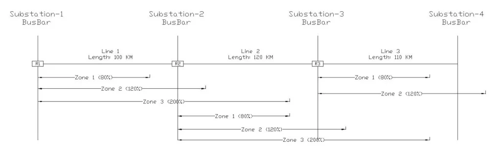
Distance Relay Coordination Example
Consider three series-connected transmission lines: Line A (200 km), Line B (180 km), and Line C (150 km).
The Line A relay at the sending end should have Zone 1 reaching 160 km at 0 ms for instantaneous protection of the primary line. Zone 2 should reach 240 km (100% of A plus 33% of B) at 0.4 s delay to provide backup for faults on the next line while allowing its Zone 1 time to operate first. Zone 3 should reach 380 km at 1.0 s delay to provide backup for faults on the second downstream line.
Line A Relay (Sending End):
- Zone 1: 160 km, 0 ms
- Zone 2: 240 km (100% A + 33% B), 0.4 s
- Zone 3: 380 km (100% A + 100% B), 1.0 s
The Line B relay at the intermediate station should have Zone 1 reaching 144 km at 0 ms for instantaneous protection of its line. Zone 2 should reach 216 km at 0.8 s delay (note the longer delay than Line A’s Zone 2 to ensure proper coordination). Zone 3 should reach 270 km at 1.4 s delay for backup to lines further downstream.
Line B Relay (Intermediate):
- Zone 1: 144 km (80% of 180), 0 ms
- Zone 2: 216 km (120% of 180 = 100% B + 20% C), 0.8 s
- Zone 3: 270 km, 1.4 s
The Line C relay at the receiving end should have Zone 1 reaching 120 km at 0 ms for instantaneous protection of its line. Zone 2 should reach 180 km at 1.2 s delay for backup to upstream lines. Zone 3 should reach 225 km at 2.0 s delay for ultimate backup.
Line C Relay (Receiving End):
- Zone 1: 120 km (80% of 150), 0 ms
- Zone 2: 180 km, 1.2 s
- Zone 3: 225 km, 2.0 s
This sequence ensures that any fault is cleared by the nearest relay first, with properly coordinated backup from upstream relays. A fault on Line B is cleared by Line B’s Zone 1 almost instantly. If that fails, Line A’s Zone 2 backs up with a 0.4 second delay. If that also fails, Line A’s Zone 3 provides ultimate protection after 1.0 second. This multi-layer backup ensures that no fault can persist on the system indefinitely.
Testing and Maintenance
Periodic Testing
Distance relays should undergo regular testing to ensure continued reliable operation.
- A Setting Verification test should be performed annually to check that all zone reaches and time delays remain within acceptable tolerances.
- CT/PT Verification tests should also be performed annually to verify that the secondary voltage and current signals are accurate and not affected by transformer saturation or other problems. Current and potential transformers that provide inputs to the relay can degrade over time, so regular verification is essential.
- More thorough Zone 1 Tests should be performed every five years by injecting fault signals at the 80% reach point to verify instantaneous operation. These tests confirm that the relay detects faults at the Zone 1 boundary and trips immediately without unexpected delays.
- Zone 2 Tests should be done every five years inject fault signals at the 120% reach point to verify time-delayed operation. These tests confirm that the relay correctly applies the 0.3-0.5 second delay and trips after the expected time.
- Additionally, Communication Tests should be performed quarterly to verify that pilot and SCADA communication links are functioning correctly if the relay uses these features. A relay that cannot communicate cannot be part of a communication-assisted protection scheme, so communication integrity is critical.
- Trip Logic Tests should be performed annually to verify that the entire tripping sequence operates correctly from fault detection through circuit breaker operation. This comprehensive testing regimen ensures that the protection system will function correctly when needed.
Distance relays should be tested at regular intervals:
| Test Type | Frequency | Method |
|---|---|---|
| Setting Verification | Annually | Check all zone reaches and time delays |
| CT/PT Verification | Annually | Verify secondary voltage/current accuracy |
| Zone 1 Test | Every 5 years | Inject fault signal at 80% reach point |
| Zone 2 Test | Every 5 years | Inject fault signal at 120% reach point |
| Communication Test | Quarterly | Verify pilot and SCADA communication |
| Trip Logic Test | Annually | Verify tripping sequence |
Conclusion
Distance protection represents the gold standard for transmission line protection due to several fundamental characteristics. The speed of instantaneous Zone 1 operation provides ultra-fast fault clearing that minimizes damage and system stress. When a fault occurs and is cleared in 30-50 milliseconds, the system barely feels the disturbance.
The selectivity of distance-based discrimination ensures that only the faulted line is disconnected, minimizing impact on healthy parts of the network. During a fault on one transmission line, all adjacent lines continue operating normally, so power continues to flow through the rest of the network.
References for Further Reading
- IEEE Std C37.113 – IEEE Guide for Protective Relay Applications to Transmission Lines
- NERC PRC Standards – Transmission System Protection Planning
- IEC 60255 Series – Electrical Relays and Protection Equipment Standards
- Power System Protective Relays – J. Lewis Blackburn
- Protective Relaying Principles and Applications – J.C. Das