Faraday’s Law of Electromagnetic Induction is one of the most foundational principles in electrical engineering and physics. Michael Faraday discovered this law in 1831 through a series of experiments. He demonstrated that a changing magnetic field can produce an electric current in a conductor.
Today, Faraday’s Law governs the operation of electric generators, transformers, electric motors, induction cooktops, wireless chargers, and numerous other devices. Every electrical engineer must develop a solid grasp of this principle to design and troubleshoot electromagnetic systems effectively.
In this technical guide, we will discuss everything you need to know about Faraday’s Law of Electromagnetic Induction, including its working principle, mathematical formulations, magnetic flux concepts, Lenz’s Law, self-inductance, mutual inductance, transformer theory, motional EMF, and real-world engineering applications. Practical examples and solved numerical problems are included throughout to help you apply these concepts in real-world scenarios confidently.
1. What is Faraday’s Law of Electromagnetic Induction?
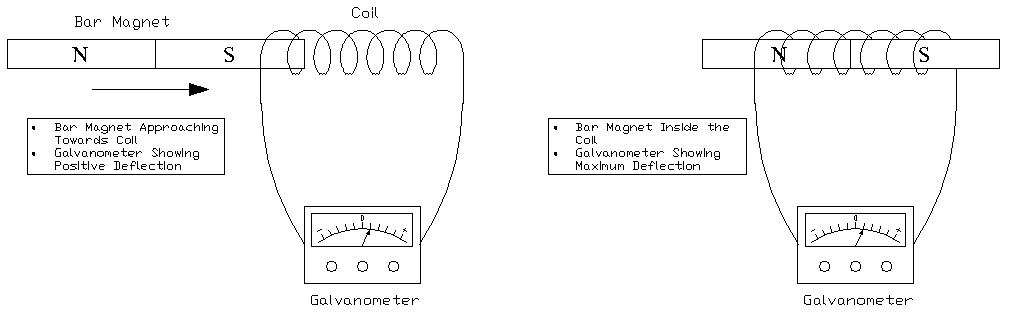
Faraday’s Law states that an electromotive force (EMF) is induced in a conductor whenever the magnetic flux through that conductor changes over time. The induced EMF is directly proportional to the rate of change of magnetic flux. Michael Faraday arrived at this conclusion after observing that moving a magnet toward or away from a coil of wire produced an electric current in the coil. This phenomenon is called electromagnetic induction.
The principle can be demonstrated through a straightforward experiment. Take a bar magnet and move it toward a coil connected to a galvanometer. The galvanometer needle deflects which indicates current flow. Move the magnet faster, and the deflection increases proportionally. The deflection reverses direction if you reverse the magnet’s motion. This simple setup illustrates the core of Faraday’s discovery.
1.1 Faraday’s First Law of Electromagnetic Induction
Faraday’s First Law gives a qualitative description of electromagnetic induction. It states that an electromotive force is induced in a conductor whenever it experiences a change in magnetic flux. If the conductor forms a closed circuit, the induced EMF drives a current through the circuit. This current is called the induced current.
The law emphasizes one fundamental requirement. There must be a change in the magnetic environment of the conductor. A static magnetic field no matter how strong will not produce any induced EMF. The change can be achieved through several methods.
Several methods can produce the required change in magnetic flux:
- Moving a magnet toward or away from a coil
- Rotating a coil inside a stationary magnetic field
- Changing the area of a coil placed within a magnetic field
- Varying the current in a nearby coil (mutual induction)
- Moving a straight conductor through a magnetic field
Each of these methods alters the magnetic flux through the conductor and results in an induced EMF according to Faraday’s Law.
1.2 Faraday’s Second Law of Electromagnetic Induction
Faraday’s Second Law provides the quantitative relationship between induced EMF and the rate of change of magnetic flux. It states that the magnitude of the induced EMF equals the rate of change of magnetic flux linkage through the coil. Flux linkage is the product of the number of turns in the coil and the magnetic flux passing through each turn.
The mathematical expression of Faraday’s Second Law is:
\( \varepsilon = -N \dfrac{d\Phi}{dt} \)
Where:
- \(\varepsilon\) is the induced electromotive force (EMF) in volts \((V)\)
- \(N\) is the number of turns in the coil
- \(\Phi\) is the magnetic flux in webers \((Wb)\)
- \(t\) is time in seconds (s)
- The negative sign represents Lenz’s Law (discussed in a later section
This equation provides several important relationships. First, increasing the number of turns in a coil increases the induced EMF proportionally. Second, a stronger magnetic field produces a greater flux change and therefore a larger EMF. Third, a faster rate of change results in a higher induced voltage.
Electrical power generation systems, electromagnetic sensors, and induction-based devices all rely on this equation for their design and analysis.
2. Magnetic Flux: The Foundation of Faraday’s Law
A solid understanding of magnetic flux is necessary before applying Faraday’s Law in calculations. Magnetic flux, denoted by \(\Phi_B\), measures the total amount of magnetic field passing through a given surface area. It quantifies how much of the magnetic field penetrates the surface and is the quantity whose change induces EMF.
The magnetic flux through a flat surface is defined mathematically as:
\( \Phi_B = B \cdot A \cdot \cos(\theta) \)
Where:
- \(\Phi_B\) is the magnetic flux measured in webers \((Wb)\) or tesla-meter squared \((T\cdot m^2)\)
- \(B\) is the magnetic field strength in teslas \((T)\)
- \(A\) is the area of the surface in square meters \((m^2)\)
- \(\theta\) is the angle between the magnetic field vector and the normal (perpendicular) to the surface
This equation shows that magnetic flux depends on three factors: field strength, surface area, and the orientation of the surface relative to the field.
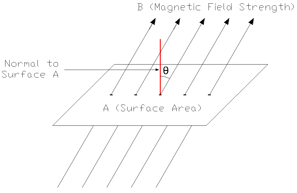
The flux reaches its maximum value of \(B\times A\) when the magnetic field is perpendicular to the surface \((\theta=0^{\circ})\), because \(\cos(0^{\circ})=1\). The flux drops to zero when the field runs parallel to the surface \((\theta=90^{\circ})\), because \(\cos(90^{\circ})=0\). At intermediate angles, the flux takes on values between these two extremes.
For non-uniform magnetic fields or irregularly shaped surfaces, the total flux must be calculated using a surface integral:
\( \Phi_B = \int_S \vec{B} \cdot d\vec{A} \)
This integral sums the magnetic field contributions over every small area element of the surface.
3. Motional EMF: Moving Conductors in Magnetic Fields
An important special case of electromagnetic induction arises when a conductor moves through a static magnetic field. This is called motional EMF. Faraday’s Law still governs this situation, but the mechanism differs slightly from the case of a time-varying field with a stationary conductor.
Consider a straight conductor of length \(L\) moving with velocity \(v\) perpendicular to a uniform magnetic field \(B\). The free electrons inside the conductor experience a magnetic force (the Lorentz force) that pushes them toward one end of the conductor. This charge separation creates a potential difference across the conductor — the motional EMF.
The motional EMF for a straight conductor moving perpendicular to both its length and the magnetic field is given by:
\(\varepsilon=B\times L \times v\)
Where:
- \(B\) is the magnetic field strength in teslas (T)
- \(L\) is the length of the conductor in meters (m)
- \(v\) is the velocity of the conductor in meters per second (m/s)
This formula assumes that the velocity, the magnetic field, and the conductor are all mutually perpendicular to each other. If they are not perpendicular, the cross product form \(\varepsilon=\int ( \vec{v} \times \vec{B})\cdot d\vec{l}\) must be used.
Motional EMF is the operating principle behind many types of electric generators and electromagnetic flow meters. It also appears in practical situations such as an airplane wing moving through the Earth’s magnetic field, which induces a small voltage across the wingspan.
4. The Maxwell-Faraday Equation
In its most general form, Faraday’s Law appears as one of Maxwell’s four equations of electromagnetism. The Maxwell-Faraday equation expresses the relationship between time-varying magnetic fields and the electric fields they produce. The differential form of this equation is:
\( \nabla \times \vec{E} = -\dfrac{\partial \vec{B}}{\partial t} \)
This equation states that a time-varying magnetic field always produces a spatially varying, circulating electric field. The curl (rotational tendency) of the electric field equals the negative time derivative of the magnetic field. This formulation applies to the fields themselves and does not require any physical conductor or circuit to be present.
The integral form of the Maxwell-Faraday equation, derived using the Kelvin-Stokes theorem, relates the circulation of the electric field around a closed loop to the rate of change of magnetic flux through the area enclosed by that loop:
\( \oint_{\partial \Sigma} \vec{E} \cdot d\vec{l} = -\iint_{\Sigma} \dfrac{\partial \vec{B}}{\partial t} \cdot d\vec{A} \)
The left side of this equation gives the EMF around the loop. The right side gives the negative rate of change of magnetic flux through any surface bounded by the loop. This integral form connects directly to practical EMF measurements in conducting loops and coils.
5. Lenz’s Law and the Negative Sign in Faraday’s Law
The negative sign in the Faraday’s Law equation carries deep physical meaning. It originates from Lenz’s Law, formulated by the Russian physicist Heinrich Lenz in 1834.
Lenz’s Law states that the induced current always flows in a direction such that its own magnetic field opposes the change in flux that produced it. This opposition is a direct consequence of the conservation of energy.
Consider what would happen if the induced current aided the flux change instead of opposing it. The increasing flux would induce more current, which would increase the flux further, creating an endless cycle of energy generation from nothing. This would violate the law of conservation of energy. Lenz’s Law prevents this situation and guarantees that external work must be done to maintain the changing flux.
Here is a practical way to determine the direction of induced current using Lenz’s Law:
- A north pole of a magnet approaches a coil. The flux through the coil increases.
- The induced current flows in a direction that creates a north pole on the side of the coil facing the magnet.
- This induced north pole repels the approaching magnet, opposing the increase in flux.
- If the magnet is pulled away instead, the flux decreases. The induced current reverses direction, creating a south pole on the near side of the coil. This south pole attracts the receding magnet, opposing the decrease in flux.
The right-hand rule serves as a practical tool here. If you curl the fingers of your right hand in the direction of the induced current, your thumb points in the direction of the magnetic field produced by that current.
6. Self-Inductance and Mutual Inductance
6.1 Self-Inductance
Self-inductance describes how a changing current in a coil induces an EMF in that same coil. As the current changes, the magnetic field produced by the coil also changes. This changing field induces an EMF in the coil that opposes the current change, consistent with Lenz’s Law.
The self-induced EMF is given by:
\( \varepsilon = -L \dfrac{dI}{dt} \)
Where \(L\) is the self-inductance (or simply inductance) of the coil, measured in henries \((H)\), and \(\dfrac{dI}{dt}\) is the rate of change of current in amperes per second (A/s).
6.2 Mutual Inductance
Mutual inductance describes the electromagnetic coupling between two nearby coils. A changing current in one coil (the primary) produces a changing magnetic field. This changing field induces an EMF in the neighboring coil (the secondary). Transformer operation is based entirely on this principle.
The mutual inductance \(M\) is defined by:
\( \varepsilon_2 = -M \dfrac{dI_1}{dt} \)
Where \(\varepsilon_2\) is the induced EMF in the secondary coil, and \(\dfrac{dI_1}{dt}\) is the rate of change of current in the primary coil.
For two magnetically coupled coils, the mutual inductance relates to their individual self-inductances through:
\( M = K\sqrt{L_1 L_2} \)
Where \(L_1\) and \(L_2\) are the self-inductances of the two coils, and \(K\) is the coupling coefficient \((0 ≤ K ≤ 1)\). A coupling coefficient of \(K=1\) indicates perfect coupling, meaning all the magnetic flux from one coil passes through the other. A value of \(K=0\) indicates no magnetic coupling between the coils. In practice, tightly wound coils on a common iron core can achieve coupling coefficients above 0.95.
7. Applications of Faraday’s Law in Electrical Engineering
Faraday’s Law governs the operation of nearly every electromagnetic device used in modern technology. From large-scale power generation to miniature electronic sensors, this principle enables the conversion between mechanical and electrical energy, voltage transformation, and many other functions that modern civilization depends upon.
7.1 Electric Generators
Electric generators are the most impactful application of Faraday’s Law. They convert mechanical energy into electrical energy and supply power to homes, industries, and infrastructure globally. A generator works by rotating a coil of wire within a stationary magnetic field, or by rotating magnets around stationary coils. As the coil rotates, the magnetic flux through it changes continuously. This changing flux induces an alternating EMF according to Faraday’s Law.
The EMF produced by an AC generator follows the equation:
\(\varepsilon=N\cdot B \cdot A \cdot \omega \cdot \sin(\omega t)\)
Where \(\omega\) is the angular velocity of rotation and \(t\) is time. The peak EMF occurs when \(\sin(\omega t)=1\). Power plants use this principle on a massive scale, with turbines driven by steam, water, wind, or gas to rotate generator shafts.
7.2 Transformers
Transformers rely on Faraday’s Law and mutual induction to transfer electrical energy between circuits at different voltage levels. A transformer consists of two coils a primary coil and a secondary coil wound around a common ferromagnetic core made of laminated steel.
Alternating current flowing through the primary coil creates a time-varying magnetic field. The core channels this magnetic flux toward the secondary coil efficiently. The changing flux induces an EMF in the secondary coil according to Faraday’s Law. The voltage ratio between the coils depends directly on their turns ratio:
\( \dfrac{V_2}{V_1} = \frac{N_2}{N_1} \)
Where \(V_1\) and \(V_2\) are the primary and secondary voltages, and \(N_1\) and \(N_2\) are the respective number of turns. A transformer with more turns in the secondary than the primary acts as a step-up transformer, increasing voltage. Fewer secondary turns create a step-down transformer, decreasing voltage.
7.3 Electric Motors and Back EMF
Electric motors convert electrical energy into mechanical energy. They operate using the magnetic force exerted on current-carrying conductors placed in a magnetic field. Faraday’s Law plays a direct role through the phenomenon of back EMF.
As a motor’s rotor spins inside the magnetic field, the changing flux through the rotor coils induces an EMF according to Faraday’s Law. This induced EMF opposes the applied voltage that drives the motor. Hence, it is called back EMF.
The back EMF is given by:
\( E_b = K_e \cdot \omega \)
Where \(E_b\) is the back EMF, \(K_e\) is the motor’s back EMF constant (specific to the motor design), and \(\omega\) is the angular velocity of the rotor. As motor speed increases, back EMF increases proportionally. At startup, the back EMF is zero, and the motor draws maximum current. As it accelerates, the back EMF rises and limits the current drawn from the supply.
7.4 Induction Cooking and Heating
Induction cooktops use Faraday’s Law to heat cooking vessels directly without heating the cooktop surface. A coil beneath the cooktop surface carries high-frequency alternating current, producing a rapidly changing magnetic field. Placing a ferromagnetic cooking vessel (such as cast iron or magnetic stainless steel) on the cooktop exposes the metal base to this changing field.
The changing magnetic flux induces eddy currents in the base of the pan. These eddy currents encounter resistance in the metal, generating heat through \(I^2 R\) losses. The pan heats up rapidly and efficiently. Induction cooking is faster and more energy-efficient than conventional gas or electric resistance cooking because heat is generated directly in the cookware.
Industrial induction furnaces use the same principle on a larger scale for melting metals and heat treatment processes.
7.5 Wireless Charging and Power Transfer
Wireless charging technology for smartphones, electric vehicles, smartwatches, and medical implants operates on electromagnetic induction as described by Faraday’s Law. A transmitter coil in the charging pad carries alternating current and generates a time-varying magnetic field. A receiver coil inside the device is placed nearby. The changing magnetic flux through the receiver coil induces an EMF, which charges the device’s battery without any physical electrical connection.
The Qi wireless charging standard, used widely in consumer electronics, operates at frequencies between 80 kHz and 300 kHz. Electric vehicle wireless charging systems use similar principles at higher power levels, with ongoing research pushing toward greater efficiency and longer-range power transfer.
7.6 Sensors and Measurement Devices
Numerous sensor technologies use electromagnetic induction based on Faraday’s Law.
Metal Detectors: A transmitter coil generates a time-varying magnetic field. Metallic objects near the detector have eddy currents induced in them. These eddy currents produce their own secondary magnetic field. A receiver coil detects this secondary field, indicating the presence and approximate location of the metal object.
Magnetic Stripe Card Readers: Credit cards and access cards store data in magnetic patterns on a stripe. Swiping the card through a reader moves the magnetic stripe past a reading head. The changing magnetic field induces voltage variations in the reader’s coil according to Faraday’s Law. These voltage patterns encode the stored information.
Electromagnetic Flow Meters: These instruments measure the flow rate of conductive fluids using Faraday’s Law. A magnetic field is applied perpendicular to the direction of fluid flow. As the conductive fluid passes through the field, an EMF is induced proportional to the flow velocity. Measuring this EMF allows accurate calculation of volumetric flow rate. Electromagnetic flow meters are used extensively in water treatment plants, chemical processing, and the oil and gas industry.
7.7 Medical Applications: MRI and Magnetic Therapy
Magnetic Resonance Imaging (MRI) machines use principles of electromagnetic induction for medical diagnostics. The primary physics of MRI involves nuclear magnetic resonance of hydrogen nuclei in the body. However, the detection of signals from these nuclei relies on Faraday’s Law directly. Precessing hydrogen nuclei produce tiny time-varying magnetic fields. These changing fields induce small voltages in receiver coils positioned around the patient. The induced voltages are amplified and processed by computers to construct detailed images of internal body structures.
MRI scanners operate with strong static magnetic fields (usually 1.5 T or 3 T) combined with gradient fields and radiofrequency pulses. The entire signal detection mechanism depends on Faraday’s Law of induction.
8. Practical Calculations and Solved Examples
8.1 Example 1: Induced EMF in a Solenoid
Problem: A solenoid of length 1 m has 200 turns and a cross-sectional area of \(2.0\times 10^-3\,m^2\). The magnetic field through the solenoid changes from 0.30 T to 0.70 T in 0.50 seconds. Calculate the magnitude of the induced EMF.
Solution:
Calculate the change in magnetic flux:
\( \Delta \Phi = \Delta B \times A \)
\(= (0.70 – 0.30) \times 2.0 \times 10^{-3}\)
\(= 0.40 \times 2.0 \times 10^{-3}\)
\( = 8.0 \times 10^{-4} Wb \)
Apply Faraday’s Law:
\( |\varepsilon| = N \frac{\Delta \Phi}{\Delta t} \)
\(= 200 \times \dfrac{8.0 \times 10^{-4}}{0.50}\)
\( = 200 \times 1.6 \times 10^{-3} = 0.32 V \)
The magnitude of the induced EMF is \(0.32\) volts.
8.2 Example 2: Magnetic Flux Through a Coil
Problem: A circular coil has a radius of 25 cm and is placed perpendicular to a uniform magnetic field of 0.5 T. Calculate the magnetic flux through the coil.
Solution:
The area of the circular coil is:
\( A = \pi r^2 = \pi \times (0.25)^2 = 0.196 m^2 \)
Since the magnetic field is perpendicular to the coil, \(\theta=0^{\circ}\) and \(\cos(0^{\circ})=1\).
The magnetic flux is:
\( \Phi_B = B \times A \times \cos(\theta) = 0.5 \times 0.196 \times 1 = 0.098 \text{Wb} \)
The magnetic flux through the coil is approximately 0.098 webers.
8.3 Example 3: Transformer Voltage Calculation
Problem: A step-up transformer has 500 turns in its primary coil and 2000 turns in its secondary coil. If the primary voltage is 120 V, calculate the secondary voltage.
Solution:
Using the transformer turns ratio equation:
\( \dfrac{V_2}{V_1} = \dfrac{N_2}{N_1} \)
Solving for \(V_2\):
\( V_2 = V_1 \times \dfrac{N_2}{N_1} = 120 \times \dfrac{2000}{500} = 120 \times 4 = 480 V \)
The secondary voltage is 480 V. This is a step-up transformer, increasing voltage by a factor of 4.
8.4 Example 4: EMF in a Moving Conductor
Problem: A straight conductor of length 0.5 m moves at a velocity of 10 m/s perpendicular to a uniform magnetic field of 0.8 T. Calculate the induced EMF.
Solution:
For a conductor moving perpendicular to a magnetic field, the induced EMF is:
\( \varepsilon = B \times L \times v = 0.8 \times 0.5 \times 10 = 4.0 V \)
The induced EMF in the moving conductor is 4.0 volts.
8.5 Example 5: Self-Induced EMF in an Inductor
Problem: An inductor with a self-inductance of 50 mH carries a current that changes at a rate of 200 A/s. Calculate the self-induced EMF.
Solution:
\( |\varepsilon|= L \dfrac{dI}{dt}=50\times 10^{−3} \times 200=10 V\)
The self-induced EMF is 10 volts. This EMF opposes the change in current, as described by Lenz’s Law.
9. Induced EMF Calculator (Faraday’s Law)
This calculator computes the induced EMF using Faraday’s Law formula: \(\varepsilon=-N\times \dfrac{\Delta\Phi}{\Delta t}\)
Inputs Required:
- Number of Turns (N)
- Initial Flux \(\Phi_1\) (Wb)
- Final Flux \(\Phi_2\) (Wb)
- Time Interval \(\Delta t\) (seconds) — must be greater than zero
Formula Applied:
\(\varepsilon=-N\times \dfrac{\Phi_2 – \Phi_1}{\Delta t}\)
The magnitude gives the induced voltage. The negative sign indicates the direction of the induced EMF per Lenz’s Law.
Induced EMF Calculator
Calculate induced EMF using Faraday’s Law: ε = -N × (ΔΦ/Δt)
10. Magnetic Flux Calculator
This calculator computes magnetic flux using the formula: \(\Phi=B\times A\times \cos(\theta)\)
Inputs Required:
- Magnetic Field \(B\) (Tesla)
- Area \(A\) (m²)
- Angle \(θ\) (degrees)
The result is given in webers (Wb).
Magnetic Flux Calculator
Calculate magnetic flux: Φ = B × A × cos(θ)
11. EMF in Moving Conductor Calculator
This calculator computes EMF in a conductor moving through a magnetic field: \(EMF=B\times L\times v\)
Inputs Required:
- Magnetic Field \(B\) (Tesla)
- Conductor Length \(L\) (meters)
- Velocity \(v\) (m/s)
This formula assumes the velocity, conductor length, and magnetic field are all mutually perpendicular.
Moving Conductor EMF Calculator
Calculate EMF in moving conductor: EMF = B × L × v
12. Conclusion
Faraday’s Law of Electromagnetic Induction remains one of the most impactful discoveries in the history of science and engineering. Michael Faraday’s experimental observations, later formalized mathematically by James Clerk Maxwell, enabled the development of virtually all modern electrical technology. The principle that a changing magnetic field induces an electromotive force provides the foundation for generators, transformers, electric motors, induction heating systems, wireless charging, electromagnetic sensors, and MRI machines.
13. Frequently Asked Questions (FAQs)
Faraday’s Law states that a changing magnetic field around a conductor induces a voltage (EMF) in that conductor. The faster the magnetic field changes, the greater the induced voltage. If the conductor is part of a closed circuit, the induced EMF drives a current through the circuit.
Faraday’s First Law is qualitative — it states that a changing magnetic field induces an EMF in a conductor. Faraday’s Second Law is quantitative — it states that the magnitude of the induced EMF equals the rate of change of magnetic flux linkage.
Lenz’s Law states that the direction of the induced current is always such that it opposes the change in magnetic flux that produced it. This law is a consequence of the conservation of energy. Without Lenz’s Law, induced currents could create energy from nothing, which would violate fundamental physics.
A transformer works on the principle of mutual induction, which is a direct application of Faraday’s Law. Alternating current in the primary coil creates a changing magnetic flux in the core. This changing flux induces an EMF in the secondary coil.
Motional EMF is the voltage induced in a conductor that moves through a static magnetic field.
Eddy currents are circulating loops of current induced in bulk conductors exposed to changing magnetic fields. They are a direct consequence of Faraday’s Law. Eddy currents produce heat and can cause energy losses in transformers and motors.
The SI unit of magnetic flux is the weber (Wb). One weber equals one tesla multiplied by one square meter (1 Wb = 1 T·m²).
Wireless chargers use a transmitter coil carrying alternating current to generate a changing magnetic field. A receiver coil in the device experiences this changing flux, and an EMF is induced according to Faraday’s Law. This induced voltage is rectified and used to charge the battery. The Qi standard for wireless charging operates at frequencies between 80 kHz and 300 kHz.
No. Faraday’s Law requires a change in magnetic flux to induce an EMF. A stationary, constant magnetic field produces zero change in flux and therefore induces no EMF.