IDMT and DMT Characteristics: Working Principle, Curve Types, Relay Settings, Coordination with Examples

Overcurrent protection is the foundation of power system protection engineering. Every electrical network needs a well-coordinated relay protection scheme to isolate faults quickly and minimize damage to equipment. Two of the most widely used relay operating characteristics in overcurrent protection are IDMT (Inverse Definite Minimum Time) and DMT (Definite Minimum Time or Definite Time). These characteristics define how a relay responds to fault current in terms of operating time.

Every protection engineer must have a solid grasp of both IDMT and DMT characteristics to design relay coordination schemes effectively.

In this technical guide, we will discuss everything you need to know about IDMT and DMT characteristics, including their working principles, types, curve equations, applications, relay settings, coordination strategies, ANSI codes, testing methods, and relevant industry standards. Practical examples are included throughout to help you apply these concepts in real-world scenarios confidently.

1. What Are Relay Time-Current Characteristics?

A time-current characteristic defines the relationship between the magnitude of fault current flowing through a relay and the time the relay takes to operate. This relationship is presented as a curve on a graph where the X-axis represents current (usually as a multiple of the pickup setting) and the Y-axis represents the operating time in seconds.

Different protection scenarios demand different time-current behaviors. In some cases, you want the relay to operate faster for higher currents. In other cases, you want the relay to wait for a fixed time before tripping, regardless of the current magnitude. This is where IDMT and DMT characteristics come into play.

The selection of the right characteristic is not arbitrary. It depends on the location of the relay in the power system, the downstream and upstream protection devices, the fault current contribution, and the equipment damage curves. A wrong selection can lead to poor coordination, nuisance tripping, or delayed fault clearance.

2. DMT Characteristics – Definite Minimum Time

2.1 Definition and Working Principle

DMT stands for Definite Minimum Time. A relay with DMT characteristics operates after a fixed, pre-determined time delay once the current exceeds the pickup value. The operating time remains constant regardless of how much the fault current exceeds the pickup setting.

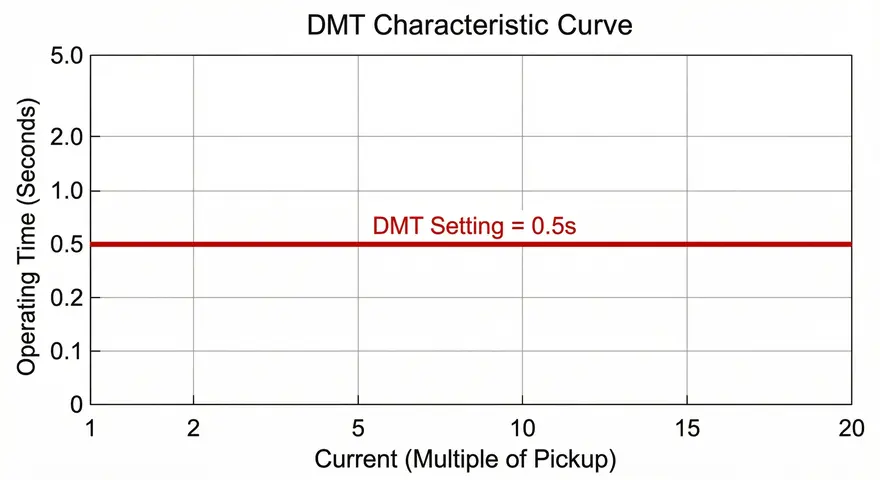
For example, if a DMT relay is set with a pickup current of 500A and a time delay of 0.5 seconds, the relay will operate in 0.5 seconds whether the fault current is 600A, 1000A, or 5000A. The only condition is that the current must exceed the 500A pickup threshold.

This behavior makes DMT relays straightforward to set and coordinate. The relay either sees a current above pickup and trips after the set time, or it does not operate at all.

2.2 DMT Characteristic Curve

The DMT time-current curve appears as a horizontal straight line on the time-current graph. Once the current crosses the pickup value, the curve remains flat at the set time delay value. Below the pickup current, the relay does not operate at all.

This flat characteristic is easy to plot and easy to understand. There is no complex mathematical equation governing the operating time. The time is simply a constant value set by the protection engineer.

2.3 How DMT Relays Are Set

Setting a DMT relay involves two parameters:

1. Pickup Current \((I_p)\): The minimum current at which the relay starts to operate. This is set based on the maximum load current and the minimum fault current at the relay location.
2. Time Delay \((t_d)\): The fixed operating time after the current exceeds the pickup value. This is selected based on the coordination time interval (CTI) with other relays in the protection scheme.

For example, in a radial distribution feeder with three relays (R1 at the load end, R2 in the middle, R3 at the source end), you might set R1 with a time delay of 0.1 seconds, R2 with 0.5 seconds, and R3 with 0.9 seconds. Each relay has a fixed time delay that increases as you move toward the source. This creates a coordinated protection scheme where the relay nearest to the fault operates first.

2.4 Advantages of DMT Characteristics

• Simple to set and coordinate
• Easy to test and verify
• Predictable operating time for all fault levels above pickup
• Works well in systems with low variation in fault current levels
• Suitable for backup protection applications

2.5 Disadvantages of DMT Characteristics

• Does not discriminate based on fault severity
• The relay near the source has a long operating time even for severe faults
• Not suitable for networks where fast fault clearance is needed for high fault currents
• Can result in excessive equipment damage during high-current faults due to fixed time delay

2.6 ANSI Code for DMT Overcurrent Relay

The ANSI/IEEE device number for a time overcurrent relay is 51. A DMT overcurrent relay uses the same ANSI code 51 but is configured with a definite time characteristic curve. For instantaneous overcurrent protection (which operates with no intentional time delay), the ANSI code is 50.

3. IDMT Characteristics – Inverse Definite Minimum Time

3.1 Definition and Working Principle

IDMT stands for Inverse Definite Minimum Time. A relay with IDMT characteristics has an operating time that decreases as the fault current increases. The word “inverse” refers to this inverse relationship between current and time. The term “definite minimum time” means that the operating time reaches a minimum value and does not decrease further beyond a certain current level.

In simple terms, an IDMT relay operates slowly for low fault currents and operates quickly for high fault currents. This behavior is highly desirable because higher fault currents indicate more severe faults that need faster isolation.

For example, if an IDMT relay has a pickup of 500A, it might take 3 seconds to operate at 600A but only 0.3 seconds to operate at 5000A. The operating time is not fixed. It depends on the ratio of the actual fault current to the pickup current setting.

3.2 The Time-Current Equation

The operating time of an IDMT relay is calculated using a standard equation defined in IEC 60255 and IEEE C37.112. The general form of the equation is:

\(t = \text{TMS} \times \frac{K}{[(\frac{I}{I_s})^\alpha – 1]}\)

Where:

• \(t\) = Operating time (seconds)
• \(\text{TMS}\) = Time Multiplier Setting (a scaling factor)
• \(K\) = A constant that depends on the curve type
• \(I\) = Actual fault current
• \(I_s\) = Pickup current setting (plug setting)
• \(\alpha\) = An exponent that depends on the curve type

The values of K and α change based on the type of inverse curve selected. This equation produces the characteristic inverse shape on the time-current graph.

3.3 Types of IDMT Curves

IDMT characteristics are available in several standard curve types. Each curve type has a different degree of “inverseness.” The main types as per IEC 60255-151 are:

3.3.1 Standard Inverse (SI)

• K = 0.14, α = 0.02
• This is the most commonly used IDMT curve
• The operating time decreases moderately with increasing current
• Used in most distribution and industrial protection schemes

3.3.2 Very Inverse (VI)

• K = 13.5, α = 1.0
• The operating time decreases more steeply with increasing current
• Suitable for systems where the fault current varies significantly between close-up and remote faults
• Often used to protect feeders with significant impedance

3.3.3 Extremely Inverse (EI)

• K = 80, α = 2.0
• The operating time drops very sharply as current increases
• Used for protecting equipment with thermal damage curves, such as transformers and motors
• Also suitable for coordinating with fuses, which have extremely inverse characteristics naturally

3.3.4 Long Time Inverse (LTI)

• K = 120, α = 1.0
• The operating time is very long at low multiples of pickup
• Used in special applications where long-time overload protection is needed

3.4 IEEE/ANSI Curve Types

The IEEE C37.112 standard defines similar curve types with slightly different constants:

• Moderately Inverse: Similar to IEC Standard Inverse
• Very Inverse: Steeper than moderately inverse
• Extremely Inverse: Steepest characteristic
• Short Time Inverse: Used for specific short-time applications
• Long Time Inverse: Used for long-duration overload conditions

The ANSI device number for IDMT overcurrent relays is also 51. The difference between DMT and IDMT implementation lies in the selected curve shape within the relay settings.

3.5 IDMT Characteristic Curve Shape

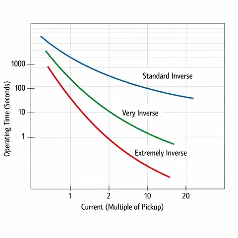
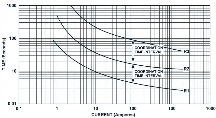
On a log-log graph, the IDMT curve appears as a line that slopes downward from left to right. At low multiples of pickup current, the curve shows a long operating time. As the current multiple increases, the curve drops steeply. At very high current multiples, the curve flattens out and approaches the definite minimum time. This minimum time is the fastest the relay can operate regardless of how high the fault current goes.

The shape of the curve varies based on the selected curve type. A Standard Inverse curve has a gentle slope. A Very Inverse curve has a steeper slope. An Extremely Inverse curve has the steepest slope among the three.

3.6 How IDMT Relays Are Set

Setting an IDMT relay requires three main parameters:

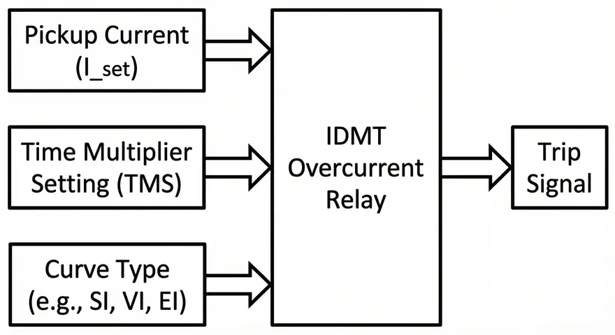
3.6.1 Plug Setting (PS) or Pickup Current

The plug setting determines the minimum current at which the relay starts to operate. It is usually expressed as a percentage of the CT secondary rated current or as an absolute current value in modern numerical relays.

Example: If the CT ratio is 400/5A and the plug setting is 100%, the pickup current is 5A on the secondary side, which corresponds to 400A on the primary side. If the plug setting is 75%, the pickup current becomes 3.75A secondary (300A primary).

The pickup current must be set above the maximum load current to avoid nuisance tripping during normal operation. A common practice is to set the pickup at 1.2 to 1.5 times the maximum load current.

3.6.2 Time Multiplier Setting (TMS)

The TMS is a scaling factor that shifts the entire IDMT curve up or down on the time axis. A higher TMS makes the relay slower. A lower TMS makes the relay faster.

TMS values range from 0.025 to 1.2 in most relays. The TMS is selected to achieve proper coordination with upstream and downstream relays.

Example: If the operating time at a specific fault current is 1.0 second with TMS = 1.0, changing the TMS to 0.5 will reduce the operating time to 0.5 seconds for the same fault current.

3.6.3 Curve Type Selection

The protection engineer selects the appropriate curve type (SI, VI, EI, or LTI) based on the application and coordination requirements.

3.7 IDMT Relay Setting Example

Consider a simple radial feeder with a relay protecting a 11kV distribution line. The following data is given:

• CT ratio: 600/5A
• Maximum load current: 450A
• Minimum fault current at the relay location: 1200A
• Maximum fault current at the relay location: 8000A

Step 1: Set the Pickup Current
Pickup = 1.3 × 450A = 585A (primary)
On secondary side: 585 × (5/600) = 4.875A
Round to nearest setting: 5.0A secondary = 600A primary

Step 2: Select the Curve Type
For a standard distribution feeder, Standard Inverse (SI) is selected.

Step 3: Calculate TMS
The TMS is calculated based on the required operating time at a specific fault level. If the downstream relay operates in 0.3 seconds for the maximum fault current, and we need a coordination time interval of 0.4 seconds, the upstream relay should operate in 0.7 seconds at the same fault current.

Using the SI formula: \(t = \text{TMS} \times \frac{0.14}{[(\frac{I}{I_s})^{0.02}– 1]}\)

At \(I = 8000A\), \(I_s = 600A\): \(\frac{I}{I_s} = 13.33\)

\(t = \text{TMS} \times \frac{0.14}{[(13.33)^{0.02} – 1]}\)
\(t = \text{TMS} \times \frac{0.14}{[1.0533 – 1]}\)
\(t = \text{TMS} \times \frac{0.14}{0.0533}\)
\(t = \text{TMS} \times 2.627\)

For \(t = 0.7\) seconds:
\(\text{TMS} = \frac{0.7}{2.627} = 0.266\)

Set \(\text{TMS} = 0.27\) (rounded to nearest available setting).

4. Differences Between IDMT and DMT Characteristics

4.1 Operating Time Behavior

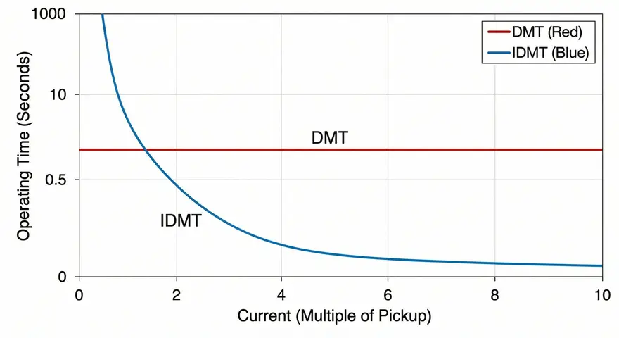
DMT relays have a constant operating time above the pickup current. IDMT relays have a variable operating time that depends on the magnitude of the fault current. This is the most fundamental difference between the two characteristics.

4.2 Fault Severity Discrimination

IDMT relays can distinguish between low-level and high-level faults by operating faster for severe faults. DMT relays treat all faults equally once the current exceeds the pickup value. This makes IDMT relays more suitable for primary protection in most applications.

4.3 Coordination Flexibility

IDMT relays offer greater flexibility in coordination because the TMS and curve type provide additional adjustable parameters. DMT relays have limited flexibility since only the pickup and time delay can be adjusted.

4.4 Application Suitability

DMT characteristics are preferred in systems where the fault current does not vary much across the protected zone. IDMT characteristics are preferred in systems with wide fault current variation, which is common in most power distribution networks.

4.5 Curve Shape

DMT curves are flat horizontal lines on the time-current graph. IDMT curves are sloping lines that decrease with increasing current.

4.6 Complexity

DMT settings are simpler to calculate and implement. IDMT settings require more detailed calculations involving the time-current equation and coordination studies.

5. Coordination of IDMT and DMT Relays

5.1 The Grading Principle

Relay coordination (also called relay grading) is the process of setting multiple relays in a protection scheme so that the relay nearest to the fault operates first. If it fails, the next upstream relay operates as backup. This is achieved by introducing time delays between successive relays.

The coordination time interval (CTI) is the minimum time difference between two successive relays. A standard CTI of 0.3 to 0.4 seconds is used in most protection schemes. This interval accounts for the circuit breaker operating time, relay overshoot time, and a safety margin.

5.2 Coordination with DMT Relays

Coordinating DMT relays is straightforward. Each relay in the chain is set with a fixed time delay that increases by the CTI value as you move from the load end toward the source.

Example:

• Relay R1 (nearest to fault): Time delay = 0.1s
• Relay R2: Time delay = 0.1 + 0.4 = 0.5s
• Relay R3 (source end): Time delay = 0.5 + 0.4 = 0.9s

The drawback is that R3 has a long operating time of 0.9 seconds even for severe faults close to its location. This can cause excessive damage to equipment at the source end.

5.3 Coordination with IDMT Relays

Coordinating IDMT relays is more complex but provides better performance. The TMS and curve type of each relay are selected so that the time-current curves of successive relays maintain the required CTI at all fault current levels.

The coordination is checked at the maximum fault current at each relay location. The upstream relay must operate at least CTI seconds slower than the downstream relay at the downstream relay’s maximum fault current level.

5.4 Mixed IDMT and DMT Coordination

In many practical protection schemes, IDMT and DMT characteristics are used together. For instance, an IDMT relay may be used for the primary overcurrent element (ANSI 51), and a DMT or instantaneous element (ANSI 50) may be used for high-set overcurrent protection.

The instantaneous element (50) provides very fast tripping for close-up faults with high fault current. The IDMT element (51) provides time-graded protection for faults further along the feeder where fault current is lower.

6. ANSI Device Numbers Related to IDMT and DMT

Here are the relevant ANSI/IEEE device numbers that protection engineers encounter when working with IDMT and DMT characteristics:

• 50 – Instantaneous Overcurrent Relay: Operates with no intentional time delay. Used for high-set overcurrent protection. This is essentially a DMT relay with zero time delay.
• 51 – AC Time Overcurrent Relay: This is the general device number for time overcurrent relays, covering both IDMT and DMT characteristics. The specific characteristic is selected within the relay settings.
• 50N/51N – Ground (Earth) Fault Overcurrent Relay: Same as 50/51 but applied to the neutral or residual current circuit for earth fault protection. Both IDMT and DMT characteristics are available.
• 50/51 – Combined Instantaneous and Time Overcurrent: Most modern numerical relays combine both elements in a single device. The instantaneous element provides fast protection for high-current faults. The time overcurrent element provides graded protection for lower-current faults.

7. Applications of DMT Characteristics

DMT characteristics are used in several specific protection applications:

7.1 Backup Protection

DMT relays serve as backup protection where the operating time is not performance-sensitive. The fixed time delay provides a reliable last line of defense.

7.2 Bus Zone Protection (Simplified)

In some busbar protection schemes, DMT relays are used to provide time-delayed backup protection for the bus section.

7.3 Directional Overcurrent with DMT

In ring main or parallel feeder configurations, directional overcurrent relays (ANSI 67) may use DMT characteristics for specific grading requirements.

7.4 Motor Protection

Some motor protection schemes use DMT elements for locked rotor protection, where the relay must trip after a defined time if the starting current persists beyond the allowed starting duration.

7.5 Breaker Failure Protection

Breaker failure protection schemes (ANSI 50BF) often use a DMT element. If the breaker fails to clear the fault within a fixed time, the breaker failure relay trips the upstream breakers.

8. Applications of IDMT Characteristics

IDMT characteristics are used more broadly across power system protection:

8.1 Distribution Feeder Protection

IDMT relays with Standard Inverse curves are the standard choice for protecting radial distribution feeders. They provide proper coordination across multiple relay stages.

8.2 Transformer Overcurrent Protection

IDMT relays protect transformers against through faults. Extremely Inverse curves are often used because they coordinate well with transformer damage curves and upstream fuses.

8.3 Generator Overcurrent Backup Protection

IDMT relays (Voltage-restrained or voltage-controlled, ANSI 51V) provide backup overcurrent protection for generators. The inverse characteristic allows the relay to ride through transient conditions.

8.4 Industrial Plant Protection

Medium voltage switchgear in industrial plants uses IDMT overcurrent relays extensively. The Very Inverse or Extremely Inverse curves are selected based on the fault current characteristics of the plant network.

8.5 Coordination with Fuses

IDMT relays with Extremely Inverse curves coordinate well with downstream fuses. Since fuses have a naturally extremely inverse characteristic, using an EI curve on the relay provides parallel time-current curves that maintain coordination across a wide current range.

8.6 Cable and Line Protection

Overhead lines and underground cables in distribution networks are protected by IDMT overcurrent relays. The curve type is selected based on the line impedance and fault current variation along the line length.

9. Testing IDMT and DMT Relays

9.1 Testing DMT Relays

Testing a DMT relay is straightforward. A secondary injection test set is used to inject current above the pickup value. The relay operating time is measured and compared with the set time delay. The test is performed at several current levels to confirm that the operating time remains constant (within tolerance) above pickup.

Test procedure:

1. Verify pickup current by slowly increasing the injected current until the relay operates
2. Inject current at 2× pickup and measure operating time
3. Inject current at 5× pickup and measure operating time
4. Inject current at 10× pickup and measure operating time
5. All operating times should be equal to the set time delay within the relay’s specified tolerance (usually ±5% or ±50ms)

9.2 Testing IDMT Relays

Testing an IDMT relay requires verifying multiple points on the time-current curve. The relay is tested at several current multiples, and the operating time at each point is compared with the theoretical time calculated from the IDMT equation.

Test procedure:

1. Verify pickup current
2. Inject current at 2× pickup and measure operating time
3. Inject current at 5× pickup and measure operating time
4. Inject current at 10× pickup and measure operating time
5. Inject current at 20× pickup and measure operating time
6. Compare measured times with calculated times from the IDMT equation
7. All points should fall within the relay manufacturer’s specified tolerance

Modern relay test sets have built-in IDMT curve equations and can automatically calculate the expected operating time for each test point. They can also generate test reports showing the deviation at each point.

10. Relevant Standards for IDMT and DMT Characteristics

Several international standards govern the design, specification, and testing of overcurrent relays with IDMT and DMT characteristics:

10.1 IEC 60255-151

This standard defines the standard IDMT curve equations and constants for Standard Inverse, Very Inverse, Extremely Inverse, and Long Time Inverse characteristics. It is the primary reference for IDMT curve definitions internationally.

10.2 IEEE C37.112

This standard defines the IDMT curve equations as used in North American practice. The curve types include Moderately Inverse, Very Inverse, Extremely Inverse, Short Time Inverse, and Long Time Inverse. The equation format differs slightly from IEC but produces similar curve shapes.

10.3 IEC 60255-1

This standard covers general requirements for measuring relays and protection equipment, including performance specifications and testing requirements.

10.4 IEEE C37.90

This standard covers relays and relay systems associated with electric power apparatus. It includes requirements for environmental testing, electromagnetic compatibility, and performance verification.

10.5 IEC 61850

Modern numerical relays that implement IDMT and DMT characteristics communicate using IEC 61850 protocols. The relay settings including curve type, pickup, and TMS are mapped to IEC 61850 logical nodes.

11. Conclusion

IDMT and DMT characteristics are the two fundamental building blocks of overcurrent protection in electrical power systems. DMT relays offer simplicity with their fixed time delay operation. They are easy to set, test, and coordinate. IDMT relays offer superior performance by adjusting their operating time based on fault severity. Higher currents result in faster tripping, which reduces equipment damage during severe faults.

Both characteristics have their place in a well-designed protection scheme. In most practical applications, IDMT and DMT elements work together within the same relay to provide layered protection. The IDMT element handles time-graded protection across a range of fault currents. The instantaneous DMT element provides fast clearance for high-current close-up faults.

12. Frequently Asked Questions (FAQs)