Transformer EMF Equation: Step-by-Step Derivation With Diagram, Formula & Solved Numerical

The EMF equation of a transformer is one of the most fundamental formulas in electrical engineering. It defines the relationship between the induced electromotive force in a transformer winding and physical parameters like frequency, magnetic flux, and number of turns. Every electrical engineer, student, or technician working with power transformers and transformer design needs to know this equation well. The transformer EMF equation E = 4.44 f N Φ appears in almost every textbook and professional examination on this subject.

In this technical guide, we will discuss everything you need to know about the transformer EMF equation, including its derivation, the origin of the 4.44 constant, primary and secondary EMF relationships, solved numerical examples, and relevant industry standards. Practical examples are included throughout to help you apply these concepts in real-world scenarios confidently.

1. What is EMF in a Transformer?

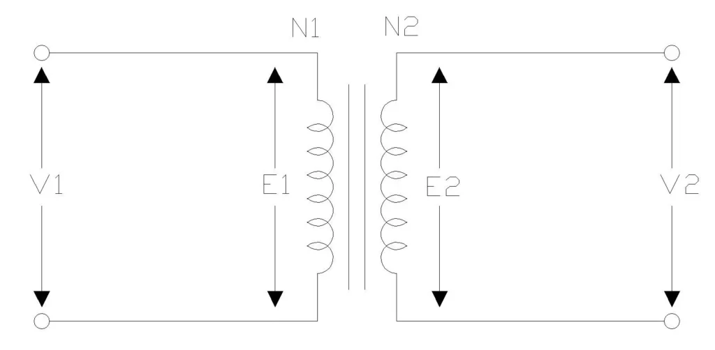
EMF stands for Electromotive Force. In a transformer, EMF is the voltage induced in the windings due to the changing magnetic flux in the core.

Think of a transformer with two coils (windings) wrapped around an iron core. The primary winding receives AC supply voltage. The secondary winding delivers the output voltage to the connected load. AC current flowing through the primary winding creates a changing magnetic flux in the iron core. This changing flux links with the secondary winding and induces an EMF in it. The magnitude of this induced EMF depends on the supply frequency, the number of turns in the winding, and the maximum magnetic flux in the core.

The same principle also applies to the primary winding itself. The changing flux induces a back-EMF in the primary, which opposes the applied voltage. This is the reason transformers draw only a small magnetizing current at no load.

2. Faraday’s Law of Electromagnetic Induction

The EMF equation is rooted in Faraday’s Law of Electromagnetic Induction. This is the starting point for the derivation of the EMF equation of a transformer. Faraday’s law states that the induced EMF in a coil equals the negative rate of change of total magnetic flux linkage through it. For a coil with N turns, the induced EMF equals N times the rate of change of flux through each turn.

Mathematically, Faraday’s law is expressed as:

\(\boxed{e = -N \dfrac{d\Phi}{dt}} \)

Where:

• \(e\) = instantaneous EMF (in volts)
• \(N\) = number of turns in the coil
• \frac{d\Phi}{dt} = rate of change of magnetic flux (in webers per second)
• The negative sign indicates Lenz’s law — the EMF opposes the change in flux

This equation forms the foundation for deriving the EMF equation of a single phase transformer. Let us now go through the step-by-step derivation.

3. Derivation of the Transformer EMF Equation

Let us derive the EMF equation of transformer with the help of the diagram shown below. This derivation explains where the famous 4.44 constant comes from and why the transformer EMF equation takes the form \(\boxed{E = 4.44 f N \Phi_{max}}\)

3.1 Step 1: Assume Sinusoidal Magnetic Flux

In AC transformers, the magnetic flux varies sinusoidally with time:

\( \Phi = \Phi_m \sin(\omega t) \)

Where:

• \(\Phi\) = instantaneous magnetic flux (in webers)
• \(\Phi_m\) = maximum (peak) magnetic flux (in webers)
• \(\omega\) = angular frequency = \(2\pi f\) (in rad/s)
• \(f\) = supply frequency (in Hz)
• \(t\) = time (in seconds)

3.2 Step 2: Apply Faraday’s Law

For the primary winding with \(N_1\) turns, the instantaneous EMF induced is:

\( e_1 = -N_1 \dfrac{d\Phi}{dt} = -N_1 \dfrac{d}{dt}(\Phi_m \sin(\omega t)) \)

Differentiating:

\( e_1 = -N_1 \Phi_m \omega \cos(\omega t) \)

Substituting \(ω = 2\pi f\):

\( e_1 = -N_1 \Phi_m (2\pi f) \cos(2\pi f t) \)

Notice the 90° phase difference between the flux (sine function) and the induced EMF (cosine function). The EMF leads the flux by 90° in a transformer.

3.3 Step 3: Find Maximum EMF

The maximum magnitude of the instantaneous EMF occurs when \(|\cos(2πft)| = 1\). The negative sign from Lenz’s law only indicates the direction of the EMF, so we take the magnitude:

\( E_{m1} = 2\pi f N_1 \Phi_m \)

Where \(E_m1\) is the maximum (peak) value of EMF in the primary winding.

3.4 Step 4: Convert to RMS Value

AC circuits use RMS (root mean square) values. For a sinusoidal waveform, the RMS value equals the peak value divided by \(\sqrt{2}\):

\( E_1 = \dfrac{E_{m1}}{\sqrt{2}} = \dfrac{2\pi f N_1 \Phi_m}{\sqrt{2}} \)

\( E_1 = \dfrac{2\pi}{\sqrt{2}} \times f \times N_1 \times \Phi_m \)

Calculating the constant:

\( \dfrac{2\pi}{\sqrt{2}} = \dfrac{6.283}{1.414} = 4.44 \)

3.5 Step 5: Final EMF Equation

The RMS value of EMF induced in the primary winding is:

\( E_1 = 4.44 \times f \times N_1 \times \Phi_m \)

Similarly, for the secondary winding:

\( E_2 = 4.44 \times f \times N_2 \times \Phi_m \)

In general form, the EMF equation of a single phase transformer is:

\(\boxed{E = 4.44 \times f \times N \times \Phi_m} \)

This completes the emf equation of transformer derivation. The equation tells us that the RMS induced voltage in any winding is directly proportional to the frequency, the number of turns, and the maximum magnetic flux in the core.

4. EMF Equation Using Flux Density

In transformer design and manufacturing, engineers often work with magnetic flux density \((B_m)\) and core cross-sectional area \((A)\) instead of total flux. The relationship between flux and flux density is:

\(\Phi_m=B_m \times A\)

Substituting this into the EMF equation gives:

\( \boxed{E = 4.44 \times f \times N \times B_m \times A} \)

Where:

• \(B_m\) = maximum magnetic flux density (in tesla, T)
• \(A\) = cross-sectional area of the core (in m²)

5. EMF Equation Parameters

The following table lists each parameter in the transformer EMF equation \(E = 4.44 f N \Phi\) along with its unit and description.

6. The 4.44 Constant — Origin and Meaning

The number 4.44 in the transformer EMF equation is not arbitrary. It comes directly from the mathematics of sinusoidal AC waveforms.

Here is how the constant is derived:

• \(2π \approx 6.283\) arises from the angular frequency and the differentiation of the sine function
• \(\sqrt{2} \approx 1.414\) comes from converting peak values to RMS values
• \(4.44 = \dfrac{2\pi}{\sqrt{2}}\) combines both factors

This constant is valid for all AC transformers operating with sinusoidal flux at any frequency. If the flux waveform is not sinusoidal, a different constant must be used.

For example, with a square wave flux, the constant becomes 4.0 instead of 4.44. The general formula uses a form factor \((K_f)\), where \(4.44 = K_f \times \pi \times \sqrt{2}\) and \(K_f = 1.11\) for a sinusoidal waveform.

7. Relationship Between Primary and Secondary EMF

Both primary and secondary windings share the same magnetic flux \((\Phi_m)\) in the core. The ratio of their induced EMFs is:

\( \dfrac{E_1}{E_2} = \dfrac{4.44 \times f \times N_1 \times \Phi_m}{4.44 \times f \times N_2 \times \Phi_m} = \dfrac{N_1}{N_2} \)

For an ideal transformer with no winding resistance or leakage flux:

\( \dfrac{E_1}{E_2} = \dfrac{N_1}{N_2} = \dfrac{V_1}{V_2} \)

Note that the relationship holds true only for an ideal transformer. In a real transformer, voltage drops across winding impedances cause the terminal voltage to differ slightly from the induced EMF.

8. EMF Per Turn

One of the most important observations from the EMF equation is that the EMF per turn is the same for both windings:

\(\dfrac{E_1}{N_1}​​=\dfrac{E_2}{N_2}​​​​=4.44\times f \times \Phi_m​\)

This happens because both windings share the same core and the same mutual flux. The EMF per turn is one of the first values a transformer design engineer calculates. It directly determines the core flux capacity and the physical size of the transformer.

For example, if a 50 Hz transformer has \(\Phi_m = 0.01 \text{Wb}\), the EMF per turn is \(4.44 \times 50 \times 0.01 = 2.22\, \text{V/turn}\).

A primary winding rated at 444 V would need \(\dfrac{444}{2.22} = 200 \,\text{turns}\).

Designers use this approach to balance between the number of turns, wire size, and core dimensions during the transformer design process.

9. Solved Numerical Problems on the EMF Equation

Let us work through practical examples to see how to apply the transformer EMF equation in real calculations.

9.1 Example 1: Calculate EMF in Both Windings

Problem: A single-phase transformer is connected to a 50 Hz supply. The maximum magnetic flux in the core is 0.0216 Wb. The primary winding has 500 turns and the secondary winding has 65 turns. Calculate the EMF induced in both windings.

Solution:

Using the EMF equation: \(E = 4.44 \times f \times N \times \Phi_m\)

For the primary winding:

\( E_1 = 4.44 \times 50 \times 500 \times 0.0216 = 2,397.6 \, \text{V}\) (approximately 2.4 kV)

For the secondary winding:

\( E_2 = 4.44 \times 50 \times 65 \times 0.0216 = 311.69 \, \text{V}\) (approximately 312 V)

Verification using turns ratio:

\( \dfrac{E_1}{E_2} = \dfrac{2,397.6}{311.69} = 7.69 \approx \dfrac{500}{65} = 7.69 \)

9.2 Example 2: Calculate Maximum Magnetic Flux

Problem: An 11,000/440 V, 50 Hz ideal single-phase transformer has a primary winding with 6,000 turns. The secondary winding is open. Calculate the maximum magnetic flux in the core.

Solution:

Given:

• \(V_1 = E_1 = 11,000 \,\text{V}\) (ideal transformer)
• \(f = 50 \,\text{Hz}\)
• \(N_1 = 6,000\,\text{turns}\)

Rearranging the EMF equation to solve for \(\phi_m\):

\( \Phi_m = \dfrac{E_1}{4.44 \times f \times N_1} \)

\( \Phi_m = \dfrac{11,000}{4.44 \times 50 \times 6,000} = 0.00826\, \text{Wb}\)

9.3 Example 3: Find Number of Primary Turns

Problem: A step-up transformer increases voltage from 440 V to 11,000 V at 50 Hz. The secondary winding has 2,500 turns. Find the number of turns in the primary winding.

Solution:

Using the transformer turns ratio equation (ideal transformer):

\( \dfrac{N_1}{N_2} = \dfrac{V_1}{V_2} \)

\( N_1 = \dfrac{V_1 \times N_2}{V_2} = \dfrac{440 \times 2,500}{11,000} \)

\( N_1 = \dfrac{1,100,000}{11,000} = 100 \)

\(N_1 = 100\, \text{turns}\)

9.4 Example 4: Find Secondary Turns and Maximum Core Flux

Problem: An ideal single-phase step-down transformer receives 400 V on its primary and supplies 230 V on its secondary. The primary has 800 turns and the supply frequency is 50 Hz. Find the number of secondary turns and the maximum core flux.

Solution:

Step 1 — Find N₂ using the turns ratio:

\( N_2 = N_1 \times \dfrac{V_2}{V_1} = 800 \times \dfrac{230}{400} = 800 \times 0.575 = 460\,\text{turns} \)

Step 2 — Find \(\Phi_m\) using the EMF equation:

For an ideal transformer at no load, \(V_1 = E_1\). Rearranging the EMF equation:

\(\Phi_m=\dfrac{E_1}{4.44\times f \times N_1} = \dfrac{400}{4.44\times 50 \times 800} = 0.00225\, \text{Wb}\) (or 2.25 mWb)

9.5 Example 5: EMF Calculation Using Flux Density and Core Area

Problem: A single-phase, 50 Hz transformer has a core with a cross-sectional area of 150 cm² and a maximum flux density of 1.2 T. The primary winding has 1,000 turns. Calculate the primary EMF.

Solution:

Given:

• \(f = 50 \,\text{Hz}\)
• \(A = 150 cm^2 = 150 \times 10^{-4} m^2 = 0.015 m^2\)
• \(B_m = 1.2 \,\text{T}\)
• \(N_1 = 1,000\, \text{turns}\)

Step 1 — Calculate \(\Phi_m\):

\(\Phi_m​=B_m​\times A=1.2\times 0.015=0.018 \,\text{Wb}\)

Step 2 — Calculate \(E_1\):

\(E_1​=4.44\times f \times N_1\times \Phi_m ​=4.44\times 50\times 1,000\times 0.018=3,996 \text{V}\)

This example shows how transformer design engineers use the flux density form of the EMF equation to determine winding requirements based on the core dimensions and material properties.

10. Important Observations from the EMF Equation

10.1 EMF is Proportional to Frequency (at Constant Flux)

If \(\Phi_m\) remains constant and you double the frequency, the induced EMF doubles:

• At 50 Hz: \(E = 4.44\times 50 \times N \times \Phi_m\)
• At 100 Hz: \(E = 4.44 \times 100 \times N \times \Phi_m\) (twice the value)

However, this only holds if the maximum flux stays the same. In practice, if a transformer is connected to a fixed voltage source and the frequency increases, \(\Phi_m\) will decrease proportionally. This is because \(V = 4.44 \times f \times N \times \Phi_m\), so if V and N are fixed, then \(f \times \Phi_m\) must remain constant. This is also the reason why 60 Hz transformers can be physically smaller than equivalent 50 Hz transformers for the same power rating.

10.2 EMF is Proportional to Number of Turns

More turns in a winding produce more EMF:

• 500 turns: \(E = 4.44 \times f \times 500 \times \Phi_m\)
• 1,000 turns: \(E = 4.44 \times f \times 1,000 \times \Phi_m\) (twice the value)

10.3 EMF is Proportional to Maximum Flux

Higher maximum flux produces more EMF. But increasing flux beyond the saturation limit of the core material is not efficient. Operating near saturation increases iron losses and introduces harmonic distortion in the flux waveform, which degrades energy efficiency.

10.4 EMF Per Turn is Constant Across Windings

For a given transformer at a fixed frequency:

\(\dfrac{​E_1}{N_1}​​=\dfrac{E_2}{N_2}​​=4.44\times f\times \Phi_m\)​

Both primary and secondary windings have the same EMF per turn because they share the same core flux.

11. Relationship Between EMF and Voltage

11.1 Ideal Transformers

In an ideal transformer with no losses:

• Primary voltage = Primary EMF \(\rightarrow V_1 = E_1\)
• Secondary voltage = Secondary EMF \(\rightarrow V_2 = E_2\)

11.2 Real Transformers

Real transformers have winding resistance and leakage reactance. The terminal voltage differs from the induced EMF:

• Primary side: \(V_1 = E_1 + (I_1\times Z_1)\) (under load)
• Secondary side: \(V_2 = E_2\, – \, (I_2 \times Z_2)\) (under load)

Here, Z is the impedance of the winding (combination of resistance R and leakage reactance X). The voltage regulation of a transformer measures how much the secondary terminal voltage drops from no-load to full-load conditions. Proper transformer testing is needed to measure actual voltage regulation performance as per industry test codes.

12. Practical Applications in Transformer Design

The EMF equation is not just a theoretical formula. Engineers in the power systems and electrical equipment industry use it daily for a number of practical tasks.

Selecting core size and material is one of the first steps. The flux density \((B_m)\) must stay below the saturation limit of the core material. For grain-oriented silicon steel (CRGO), this limit is about 1.5 T to 1.7 T. The EMF equation directly links the required core area to the voltage rating and number of turns.

Determining the turns count is another direct application. For a given voltage rating, frequency, and core flux, the required number of turns can be calculated from the equation. This is done for both primary and secondary windings.

Frequency compatibility is also governed by the EMF equation. A transformer designed for 50 Hz will have more turns than an equivalent 60 Hz transformer. If a 50 Hz transformer is accidentally connected to a 60 Hz supply, the flux will be lower (since Φ_m = V / 4.44fN), which reduces core losses but slightly changes the voltage ratio. Operating a 60 Hz transformer on a 50 Hz supply is more dangerous because it increases the flux, pushing the core toward saturation.

Voltage ratio design in power distribution systems relies directly on the turns ratio derived from the EMF equation. Transmission transformers that step up voltage for long-distance power transmission and distribution transformers that step it down for consumer use are both designed using this same equation.

13. Relevant Industry Standards

The design, testing, and performance of power transformers in the United States and other countries are governed by several ANSI and IEEE standards. These standards define the testing methods, performance criteria, and terminology used across the transformer industry.

14. Important Points to Remember

15. Conclusion

The transformer EMF equation \(E = 4.44 \times f \times N \times \Phi_m\) is a direct result of Faraday’s law applied to sinusoidal AC systems. It tells you how much voltage a transformer can induce based on the supply frequency, the number of winding turns, and the maximum core flux. The 4.44 constant comes from 2π/√2 and is valid only for sinusoidal waveforms.

This formula is the foundation of all transformer design and analysis work in the electrical engineering field. Engineers use it daily to select core sizes, calculate winding turns, and verify voltage ratings. A solid command of this equation and its derivation will serve you well in any power systems career from transformer design and electrical equipment testing to industrial transformer maintenance and power distribution planning.

16. Frequently Asked Questions