B-H Curve of Magnetic Materials: Theory, Hysteresis Loss, Practical Examples, and Standards

The B-H curve is one of the most fundamental concepts in electromagnetism and magnetic circuit design. Every electrical engineer encounters this curve while studying transformers, inductors, electric motors, and other magnetic devices. The B-H curve describes the relationship between magnetic flux density (B) and magnetic field intensity (H) in a magnetic material. It tells us how a material responds to an applied magnetic field and helps engineers select the right core material for a specific application. Without a proper grasp of the B-H curve, designing efficient electrical machines and power systems becomes extremely difficult.

In this technical guide, we will discuss everything you need to know about the B-H curve, including its working principle, different regions, hysteresis loop, types of magnetic materials, applications in electrical engineering, relevant industry standards, and practical examples.

1. What Is the B-H Curve?

The B-H curve is a graphical representation that shows how a magnetic material responds when it is subjected to an external magnetic field. The horizontal axis represents the magnetic field intensity (H), measured in Amperes per meter (A/m). The vertical axis represents the magnetic flux density (B), measured in Tesla (T).

The curve starts from the origin for a fresh, unmagnetized sample. As the magnetic field intensity increases, the flux density also increases. Initially, the increase is steep because the magnetic domains within the material align quickly with the external field. After a certain point, the curve starts to flatten. This flattening indicates that the material is approaching magnetic saturation. At saturation, almost all the magnetic domains are aligned, and further increases in H produce very little change in B.

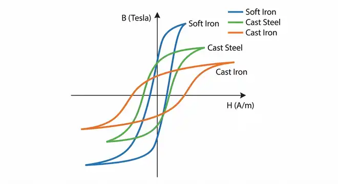
The shape of the B-H curve varies from material to material. Soft magnetic materials like silicon steel have a steep and narrow curve. Hard magnetic materials like alnico have a wide curve. This distinction is extremely useful for engineers working on transformer core design, permanent magnet selection, and electromagnetic device optimization.

2. The Physics Behind the B-H Curve

To fully understand the B-H curve, you need to know what happens inside a magnetic material at the atomic level. Every atom in a ferromagnetic material acts like a tiny magnet due to the spin of its electrons. Groups of atoms with aligned magnetic moments form regions called magnetic domains.

In an unmagnetized state, these domains are randomly oriented. The net magnetic effect cancels out, and the material shows no external magnetism. Once an external magnetic field is applied, the domains start to align in the direction of the field. This alignment causes the flux density (B) to rise.

The relationship between B and H is governed by the equation:

\(\boxed{B = \mu \times H}\)

Here, \(\mu\) is the permeability of the material. Permeability is not a constant value for ferromagnetic materials. It changes depending on the level of magnetization. This non-linear behavior is exactly what the B-H curve captures.

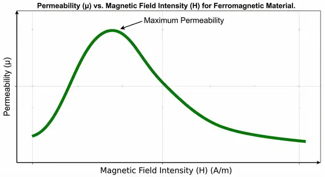
At low values of H, permeability is moderate. As H increases, permeability rises and reaches a maximum value. Beyond that point, permeability decreases as the material approaches saturation. This variation in permeability is why the B-H curve is non-linear for ferromagnetic materials.

3. Different Regions of the B-H Curve

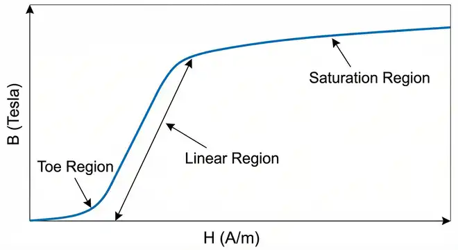
The B-H curve can be divided into three distinct regions. Each region represents a different phase of the magnetization process.

3.1 Initial Region (Toe Region)

At the very beginning of the curve, a small increase in H produces a relatively small increase in B. The magnetic domains that are most favorably oriented begin to grow at the expense of less favorably oriented domains. The curve rises slowly in this region.

3.2 Linear (Steep) Region

In this region, the curve rises sharply. A moderate increase in H leads to a large increase in B. Domain walls move rapidly, and many domains rotate to align with the applied field. The permeability of the material is at its highest in this region. This is the most efficient operating region for most electrical machines and transformers. Engineers design magnetic circuits to operate within this zone to achieve maximum energy efficiency.

3.3 Saturation Region

Beyond a certain value of H, the curve flattens out. Nearly all domains are aligned with the external field. Any further increase in H produces only a very marginal increase in B. Operating in this region is generally undesirable because it leads to high magnetizing currents, increased core losses, and reduced efficiency. Transformer and motor designers avoid pushing the core material into deep saturation under normal operating conditions.

4. The Hysteresis Loop

The B-H curve becomes even more interesting when you consider the complete cycle of magnetization and demagnetization. If you increase H to saturation, then reduce it back to zero, and then reverse the direction of H, the B-H curve does not retrace its original path. Instead, it forms a closed loop called the hysteresis loop.

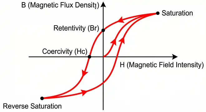
4.1 Retentivity (Residual Magnetism)

When the external field H is reduced to zero after magnetization, the flux density B does not return to zero. The value of B that remains is called retentivity or remanence (Br). This residual magnetism is the reason permanent magnets exist. Materials with high retentivity are suitable for making permanent magnets.

4.2 Coercivity

To bring the flux density B back to zero, you must apply a reverse magnetic field. The magnitude of this reverse field is called coercivity (Hc). Materials with high coercivity are hard to demagnetize. Hard magnetic materials have high coercivity values, making them ideal for permanent magnets. Soft magnetic materials have low coercivity, which means they can be easily magnetized and demagnetized. This property makes soft materials ideal for transformer cores and motor laminations.

4.3 Hysteresis Loss

The area enclosed by the hysteresis loop represents the energy lost per unit volume per cycle. This energy is dissipated as heat within the core material. In power transformers operating at 50 Hz or 60 Hz, the core goes through thousands of magnetization cycles every minute. Minimizing hysteresis loss is a primary concern in power system design and energy-efficient electrical equipment manufacturing.

The hysteresis loss can be calculated using the Steinmetz equation:

\(\boxed{P_h = \eta \times B_{max}^n \times f \times V}\)

Where:

• \(P_h\) = Hysteresis loss (Watts)
• \(\eta\) = Steinmetz hysteresis coefficient (depends on the material)
• \(B_{max}\) = Maximum flux density (Tesla)
• \(n\) = Steinmetz exponent (between 1.5 and 2.5)
• \(f\) = Frequency \((Hz)\)
• \(V\) = Volume of the core \((m^3)\)

5. Types of Magnetic Materials and Their B-H Curves

Different materials exhibit very different B-H curve characteristics. The three major categories are diamagnetic, paramagnetic, and ferromagnetic materials.

5.1 Diamagnetic Materials

Diamagnetic materials like copper, silver, and bismuth have a nearly flat B-H curve with a slope slightly less than that of free space. They weakly oppose the applied magnetic field. Their permeability is slightly less than \(\mu_{0}\) (permeability of free space). These materials are not used in magnetic circuit design.

5.2 Paramagnetic Materials

Paramagnetic materials like aluminum, platinum, and tungsten have a B-H curve with a slope slightly greater than free space. They are weakly attracted to the magnetic field. Their permeability is slightly greater than \(\mu_{0}\). Like diamagnetic materials, they have limited use in electromagnetic device design.

5.3 Ferromagnetic Materials

Ferromagnetic materials like iron, cobalt, nickel, and their alloys have steep, non-linear B-H curves with very high permeability. These are the materials used in transformers, motors, generators, inductors, and relays. Ferromagnetic materials are further divided into soft and hard categories.

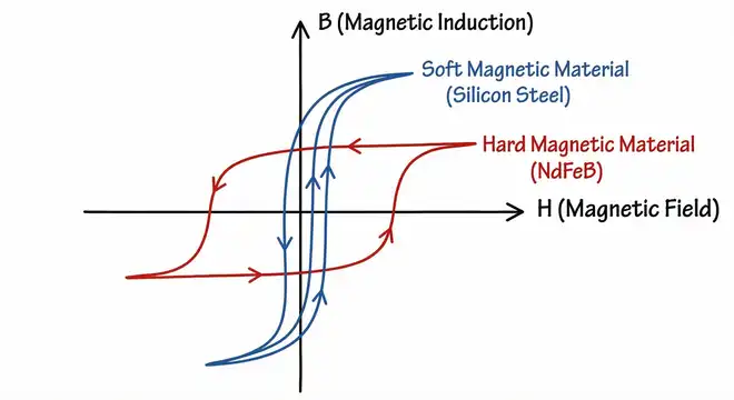
5.3.1 Soft Magnetic Materials

• Silicon steel (electrical steel)
• Mumetal
• Ferrites (for high-frequency applications)
• Amorphous metals

Soft materials have narrow hysteresis loops, low coercivity, and low hysteresis losses. They are used in power transformer cores, distribution transformer cores, motor stator and rotor laminations, and choke coils.

5.3.2 Hard Magnetic Materials

• Alnico
• Neodymium Iron Boron (NdFeB)
• Samarium Cobalt (SmCo)
• Ferrite magnets

Hard materials have wide hysteresis loops, high coercivity, and high retentivity. They are used in permanent magnets, loudspeakers, magnetic storage media, and electric vehicle motors.

6. Permeability and the B-H Curve

Permeability \((\mu)\) is the measure of how easily a material can be magnetized. It is derived directly from the B-H curve.

Absolute Permeability: \(\mu = \dfrac{B}{H}\)

Relative Permeability: \(\mu_r =\dfrac{\mu}{\mu_0}\)

Where \(\mu_0 = 4\pi \times 10^{-7} \, H/m\) (permeability of free space)

For ferromagnetic materials, permeability is not constant. It changes along the B-H curve. At low H values, permeability is moderate. It increases as H increases through the steep region of the curve. It reaches a peak and then decreases as the material enters saturation.

Engineers often use two types of permeability:

1. Initial Permeability \((\mu_i)\): The slope of the B-H curve at the origin. This value is important for small-signal applications and sensor design.
2. Maximum Permeability \((μ_{max})\): The steepest slope on the B-H curve. This value indicates the most efficient operating point of the material.

7. Practical Example: Selecting a Transformer Core Material

Let us walk through a practical example to illustrate how the B-H curve guides engineering decisions.

Suppose you are designing a 50 Hz, 10 kVA single-phase power transformer. You need to choose a core material that minimizes losses and operates efficiently at the rated flux density.

Step 1: Determine the operating flux density. For grain-oriented silicon steel (GOES), a common operating flux density is 1.5 T to 1.7 T at 50 Hz. The B-H curve for GOES shows that this range falls within the steep portion of the curve, just before saturation begins.

Step 2: Check the magnetizing force required. From the B-H curve of M4-grade GOES, at B = 1.7 T, the required H is approximately 100 A/m. This is a reasonable value and means the transformer will not need excessive magnetizing current.

Step 3: Evaluate hysteresis loss. M4-grade GOES has a narrow hysteresis loop. The core loss (including hysteresis and eddy current losses) at 1.7 T and 50 Hz is approximately 1.0 to 1.3 W/kg. This is acceptable for a high-efficiency transformer.

Step 4: Check the saturation point. The B-H curve shows that GOES saturates around 2.0 T. Operating at 1.7 T gives a safety margin of about 15-18% before reaching saturation. This margin protects the transformer during voltage surges and transient overloads.

8. B-H Curve in Electrical Machine Design

The B-H curve plays a central role in the design of rotating electrical machines such as induction motors, synchronous generators, and brushless DC motors.

8.1 Induction Motors

In an induction motor, the stator and rotor cores are made from laminated silicon steel. The B-H curve of the lamination material determines the maximum flux density in the air gap, stator teeth, stator yoke, rotor teeth, and rotor yoke. Designers use the B-H curve to calculate the magnetomotive force (MMF) required for each section of the magnetic circuit. If any section operates in the saturation region, the motor will draw excessive magnetizing current and its power factor will drop.

8.2 Synchronous Generators

In synchronous generators used in power plants, the rotor field winding produces the main magnetic flux. The B-H curve of the rotor and stator core materials determines how much field current is needed to achieve the desired terminal voltage. Generator designers use the B-H curve data in conjunction with the open-circuit characteristic (OCC) to predict the machine’s voltage regulation and excitation requirements.

8.3 Permanent Magnet Motors

In permanent magnet motors used in electric vehicles and industrial servo drives, the B-H curve of the permanent magnet material (such as NdFeB) determines the operating point of the magnet. The second quadrant of the hysteresis loop, known as the demagnetization curve, is especially important. It shows how the magnet performs under load and whether it can withstand demagnetizing fields without losing its magnetism permanently.

9. B-H Curve and Core Losses in Power Systems

Core losses are a major concern in power transformers, distribution transformers, and voltage regulators. These losses occur continuously as long as the transformer is energized, regardless of the load. Core losses consist of two components:

9.1 Hysteresis Loss

As explained earlier, hysteresis loss is proportional to the area of the hysteresis loop. Materials with narrow loops (low hysteresis loss) are preferred for power frequency applications. Grain-oriented silicon steel is the industry standard for large power transformers because of its exceptionally narrow hysteresis loop in the rolling direction.

9.2 Eddy Current Loss

Eddy current loss is caused by circulating currents induced in the core by the alternating magnetic flux. Although eddy current loss is not directly visible on the B-H curve, the choice of core material and lamination thickness are influenced by the B-H characteristics. Thinner laminations and higher resistivity materials reduce eddy current losses.

The total core loss is often specified by manufacturers in data sheets as a function of flux density and frequency. For example, a manufacturer might specify that M3-grade GOES has a total core loss of 0.97 W/kg at 1.7 T and 50 Hz. This information, combined with the B-H curve, allows engineers to design transformers that meet energy efficiency standards such as ANSI/IEEE C57.12.00 and DOE 10 CFR Part 431.

10. Relevant Industry Standards

Several industry standards reference the B-H curve and magnetic material properties. Here are some of the most important ones:

• ASTM A340: Standard Terminology of Symbols and Definitions Relating to Magnetic Testing. This standard defines terms like retentivity, coercivity, permeability, and hysteresis loss.
• ASTM A343 / A343M: Standard Test Method for Alternating-Current Magnetic Properties of Materials at Power Frequencies Using Wattmeter-Ammeter-Voltmeter Method and 25-cm Epstein Frame.
• ASTM A596: Standard Test Method for Direct-Current Magnetic Properties of Materials Using the Ballistic Method and Ring Specimens.
• ANSI/IEEE C57.12.00: IEEE Standard for General Requirements for Liquid-Immersed Distribution, Power, and Regulating Transformers. This standard includes specifications for core loss limits that are directly related to B-H curve properties.
• IEC 60404: Series of international standards covering magnetic materials, including measurement methods for B-H curves and core loss characteristics.
• NEMA MG 1: Motors and Generators. This standard references magnetic circuit design practices that depend on B-H curve data.

11. How to Measure the B-H Curve

The B-H curve of a material can be measured using several experimental methods. The most common methods include:

11.1 Epstein Frame Test

The Epstein frame test is the industry standard method for measuring the magnetic properties of electrical steel. It uses a square frame made of four bundles of test strips. A primary winding applies the magnetizing force (H), and a secondary winding measures the induced voltage, from which the flux density (B) is calculated. This method is described in ASTM A343 and IEC 60404-2.

11.2 Ring Specimen Test

In this method, a toroidal ring sample is wound with a primary and secondary winding. The advantage of the ring test is that it eliminates air gaps and provides a uniform magnetic path. The ring test is described in ASTM A596 and is preferred for measuring DC B-H curves.

11.3 Single Sheet Tester (SST)

The SST method uses a single sheet of the test material placed between two yokes. It is faster and requires less sample material than the Epstein frame. The SST method is described in IEC 60404-3.

11.4 Vibrating Sample Magnetometer (VSM)

A VSM measures the B-H curve of small material samples by vibrating them in a magnetic field and detecting the induced voltage in pickup coils. This method is commonly used in research laboratories for characterizing new magnetic materials and permanent magnets.

12.Example: Calculation of Flux Density in a Magnetic Circuit

Let us work through a numerical example.

Problem: A toroidal core made of cast steel has a mean magnetic path length of \(0.5\, m\) and a cross-sectional area of \(4 \times 10^{-4} m^2\). A coil of 200 turns is wound on the core. The coil carries a current of 2 A. Using the B-H curve for cast steel, determine the flux density and the total magnetic flux in the core.

Solution:

Step 1: Calculate the magnetic field intensity (H).

\(H = \dfrac{NI}{l} = \dfrac{(200 \times 2)}{0.5} = 800\, A/m\)

Step 2: From the B-H curve of cast steel, at H = 800 A/m, the corresponding flux density B is approximately 1.2 T.

Step 3: Calculate the total magnetic flux \((\Phi)\).

\(\Phi = B \times A = 1.2 \times 4 \times 10^{-4} = 4.8 \times 10^{-4} Wb = 0.48\, mWb\)

13. Conclusion

The B-H curve is a foundational tool in electrical engineering that connects the applied magnetic field intensity to the resulting magnetic flux density in a material. It guides engineers in selection of core materials, designing transformers, building electric motors, and optimizing power electronic circuits. The hysteresis loop, an extension of the B-H curve, reveals the energy losses within magnetic materials during cyclic magnetization.

Engineers who master the B-H curve can make informed decisions about material selection, operating flux density, loss minimization, and overall system efficiency. From large power transformers in utility substations to tiny ferrite inductors in smartphone chargers, the B-H curve remains an indispensable reference for every magnetic circuit design.

14. Frequently Asked Questions (FAQs)